HadISDH Figures from Willett et al., (2014)

Please read the paper before using the material presented here.

All figures have been created using HadISDH.land*.2.0.0.2013p and are under Crown Copyright. Please acknowledge use of this material using the following reference:

Willett, K. M., Dunn, R. J. H., Thorne, P. W., Bell, S., de Podesta, M., Jones, P. D., Parker D. E. and Williams Jr., C. N.,submitted.: HadISDH land surface multi-variable humidity and temperature record for climate monitoring. Climate of the Past.
Open Access pdf and Supplementary material

Title	Description	Link
Figures from Willett et al. 2014
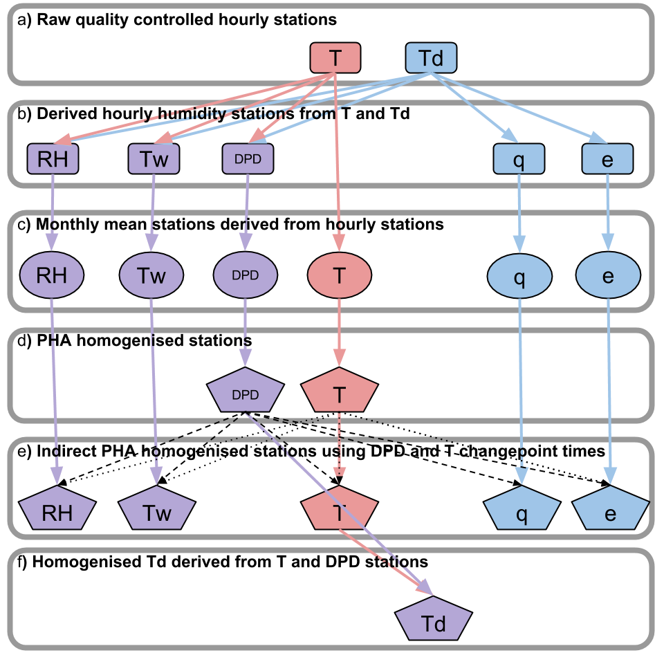
Fig. 1 HadISDH Processing	Flow diagram of HadISDH.2.0.0 processing from hourly quality-controlled values to monthly mean homogenised station values.	Fig1_HadISDH.2.0.0Process_v1.png
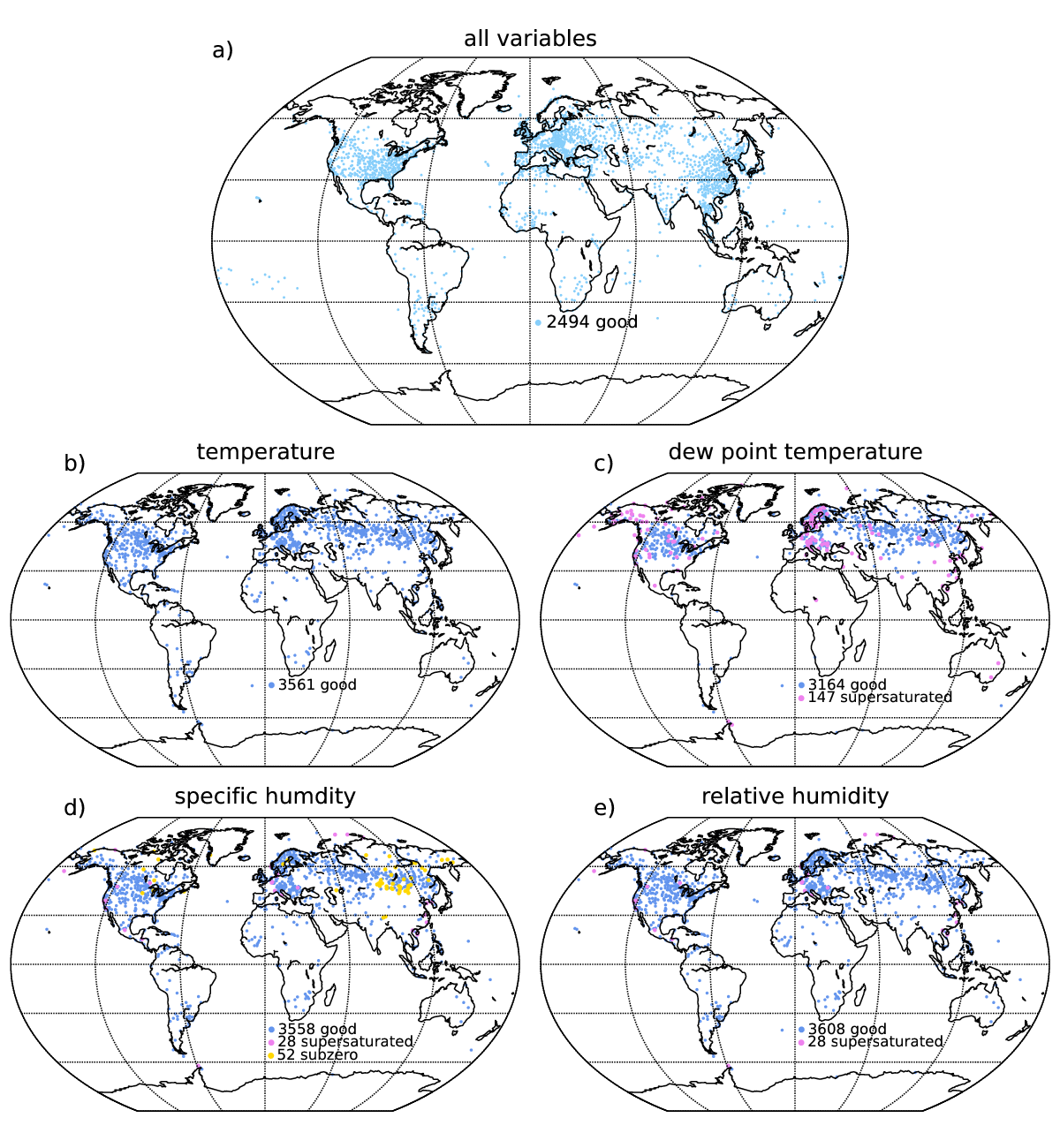
Fig. 2 Station coverage	Final station coverage maps with supersaturated and subzero error stations identified that are not included in the final HadISDH data sets. (a) Good stations common to all variables, (b) additional temperature stations, (c) additional dew point temperature stations, (d) additional specific humidity stations, and (e) additional relative humidity stations. See Fig. SM1 for other variables.	Fig2_StationLocationsDiffs.landALL.2.0.0.2013p_SEP2014_v1.png
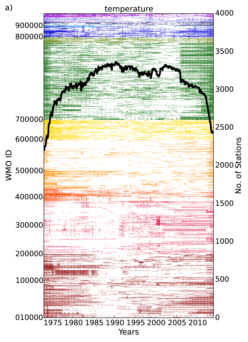
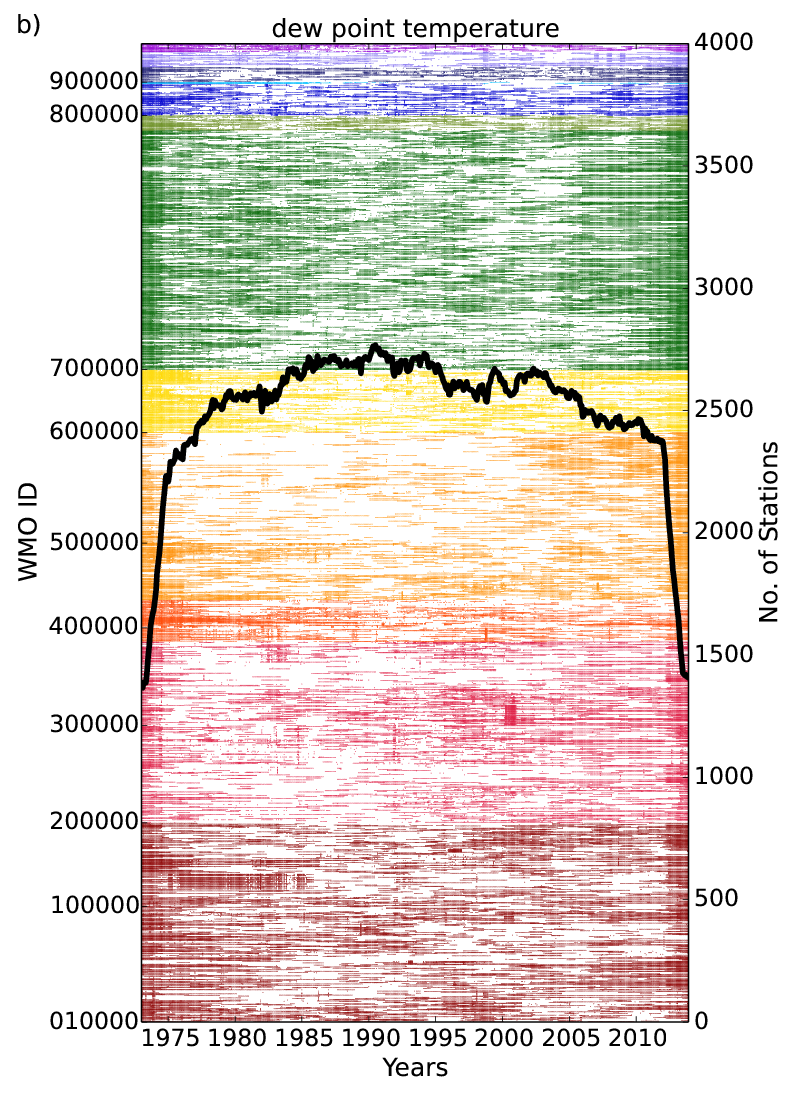
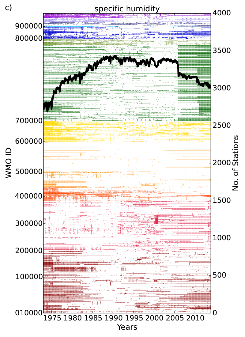
Fig. 3 Station temporal coverage	Station temporal coverage. Colours show missing station months by WMO ID (left y-axis) and the solid black line shows total station count (right y-axis). WMO IDs/colours are bounded as follows: Europe: 0-199999 (dark red), Russia/Eastern Europe: 200000-379999 (crimson), Central Asia/Middle East/India/Pakistan: 380000-439999 (dark orange), South East Asia/East Asia/China: 440000-599850 (orange), Africa: 600000-689999 (gold), USA/Canada: 690000-749 999 (dark green), Central America: 760000-799999 (olive green), South America: 800000-879999 (royal blue), Antarctica: 880000-899999 (sky blue), Pacific Islands (Inc. Hawaii): 911000-919999 (navy), Papua New Guinea/Australia/New Zealand: 930000-949999 (lilac), Indonesia/Philippines/Borneo: 960000-999999 (purple). (a) Temperature, (b) dew point temperature, (c) specific humidity and (d) relative humidity. See Fig. SM2 for other variables.	Fig3a_TemporalCoverage.landT.2.0.0.2013p_SEP2014INV_v1.png, Fig3b_TemporalCoverage.landTd.2.0.0.2013p_SEP2014INV_v1.png, Fig3c_TemporalCoverage.landq.2.0.0.2013p_SEP2014INV_v1.png, Fig3d_TemporalCoverage.landRH.2.0.0.2013p_SEP2014INV_v1.png
Fig. 4 Pagri, Tibet	Example of an inhomogeneity having a greater signal-to-noise ratio in DPD compared to q for station 557 730, Pagri, Tibet. (a) DPD annual mean series for raw data (red) and direct PHA homogenised data (blue) for 557730 and its raw neighbour series (black). (b) q annual mean series for raw data (red) and direct PHA homogenised data (blue) for 557730 and its raw neighbour series (black). (c) q annual mean series for raw data (red) and indirect PHA homogenised data (blue) for 557730 and its raw neighbour series (black).	Fig4a_55773099999_trendcompPHAdpd_7313SEP2014abs_v1.png, Fig4b_55773099999_trendcompPHAq_7313SEP2014abs_v1.png, Fig4c_55773099999_trendcompIDPHAq_7313SEP2014abs_v1.png
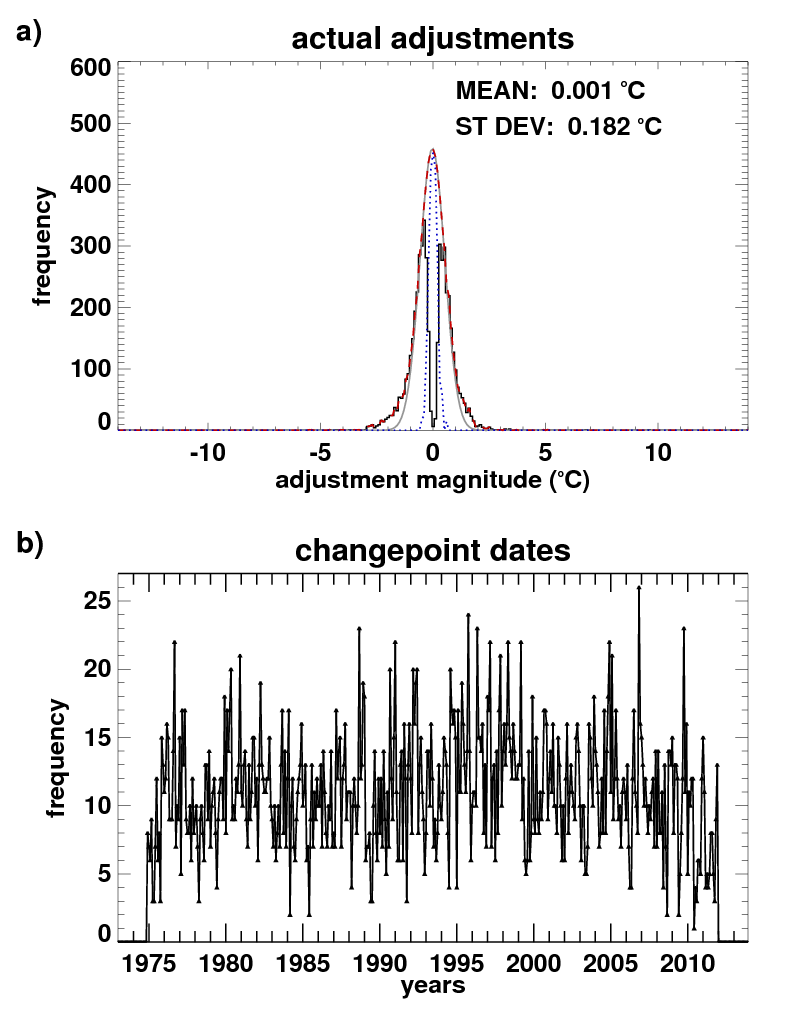
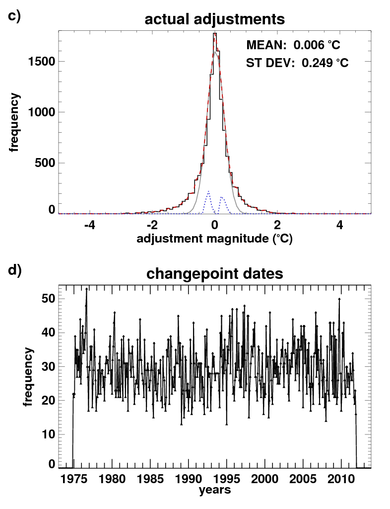
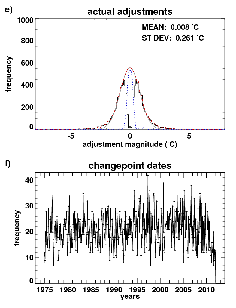
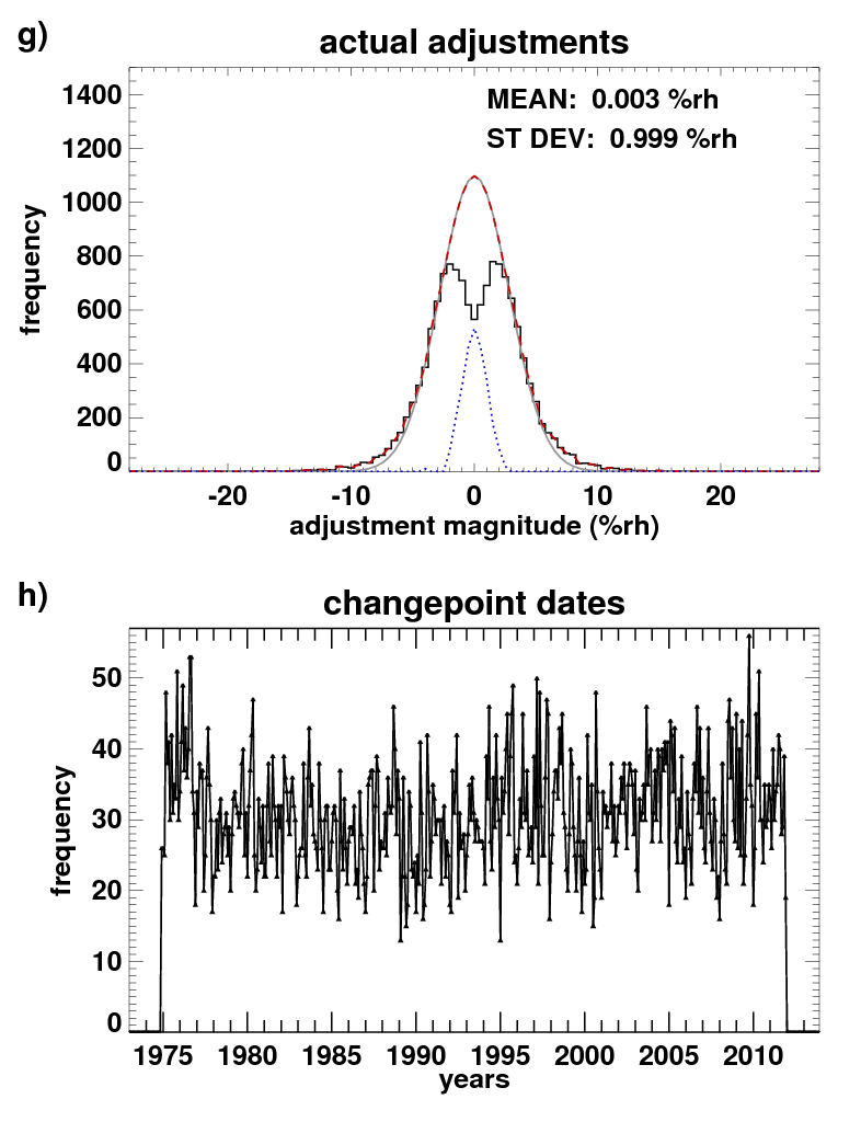
Fig. 5 Homogeneity adjustment frequency and magnitude	Adjustment sizes and locations applied by PHA (a, b, e, f) and ID PHA (c, d, g, h) to all monthly mean station time series combined. (a, c, e, g) Distribution of adjustment size (black line) with a Gaussian fit (grey line), a best-fit merged line taking the larger wings and Gaussian fit over the missing middle (red dashed line) and the difference between the best-fit line and actual distribution (blue dotted line) for temperature, dew point depression and relative humidity, respectively. The mean and standard deviation of the differences are shown. b,d,f,h) Distribution of adjustments over time for temperature (a, b, c, d), dew point depression (e, f) and relative humidity (g, h), respectively.	Fig5ab_HadISDH.landT.2.0.0.2013p_adjspread_PHA_SEP2014_v1.png, Fig5cd_HadISDH.landT.2.0.0.2013p_adjspread_IDPHAMG_SEP2014_v1.png, Fig5ef_HadISDH.landDPD.2.0.0.2013p_adjspread_PHA_SEP2014_v1.png, Fig5gh_HadISDH.landRH.2.0.0.2013p_adjspread_IDPHA_SEP2014_v1.png
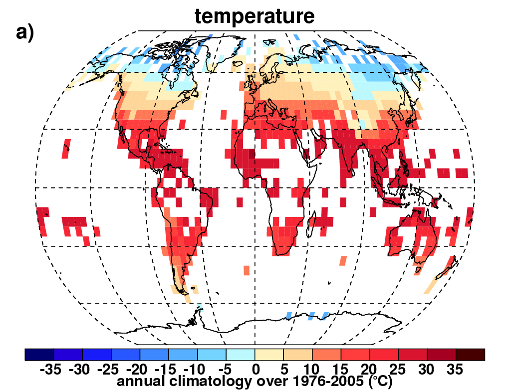
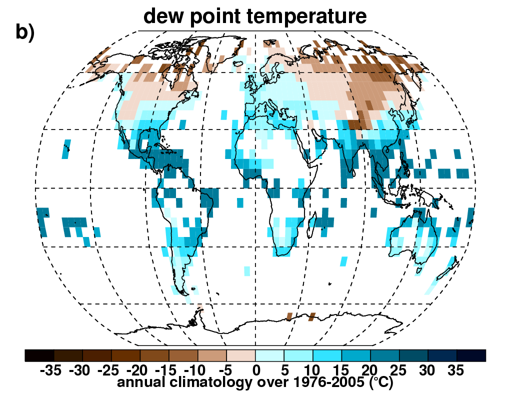
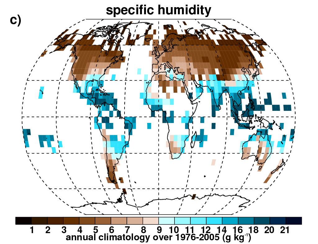
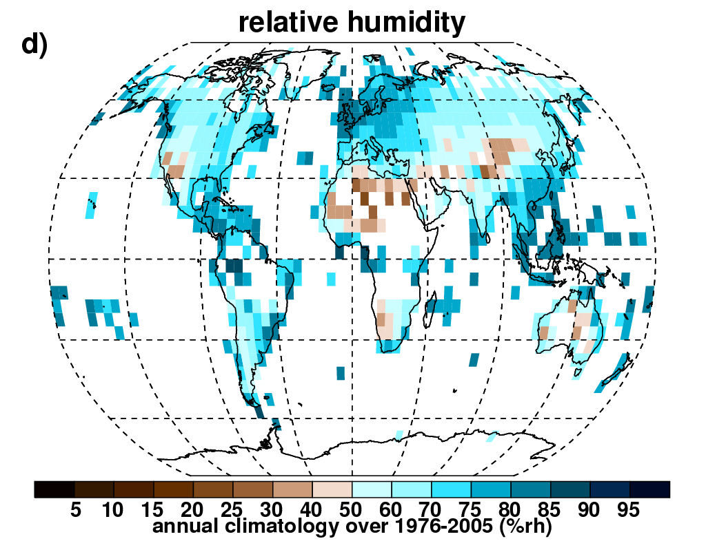
Fig. 6 Annual climatologies	Annual climatologies (1976-2005) for (a) temperature, (b) dew point temperature, (c) specific humidity and (d) relative humidity. See Fig. SM5 for other variables.	Fig6a_HadISDH.landT.2.0.0.2013p_FLATgridIDPHA5by5_SEP2014_climsANN7605_v1.png, Fig6b_HadISDH.landTd.2.0.0.2013p_FLATgridPHADPD5by5_SEP2014_climsANN7605_v1.png, Fig6c_HadISDH.landq.2.0.0.2013p_FLATgridIDPHA5by5_SEP2014_climsANN7605_v1.png, Fig6d_HadISDH.landRH.2.0.0.2013p_FLATgridIDPHA5by5_SEP2014_climsANN7605_v1.png
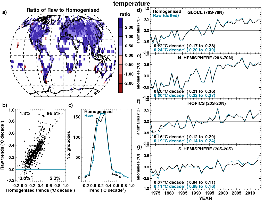
Fig. 7 Comparing raw and homogenised trends in temperature	Comparison of decadal trends from 1973-2013 between raw and homogenised monthly mean temperature. (a) Ratio of raw to homogenised trends for each grid box (a value of > 1 means that the raw trend is greater than the homogenised trend). (b) Scatter plot of raw verses homogenised decadal trends for each grid box with percentage presence in each quadrant. (c) Trend size distribution for raw and homogenised grid boxes. (d) Large-scale area-average time series (weighted by the cosine of the latitude) and decadal trends calculated using the median of pairwise slopes with 5th to 95th percentile slopes as con?dence intervals.	Fig7_HadISDH.landT.2.0.0.2013p_FLATgridIDPHA5by5_MAY2014_MPtrendsscat_19732013_v1.png
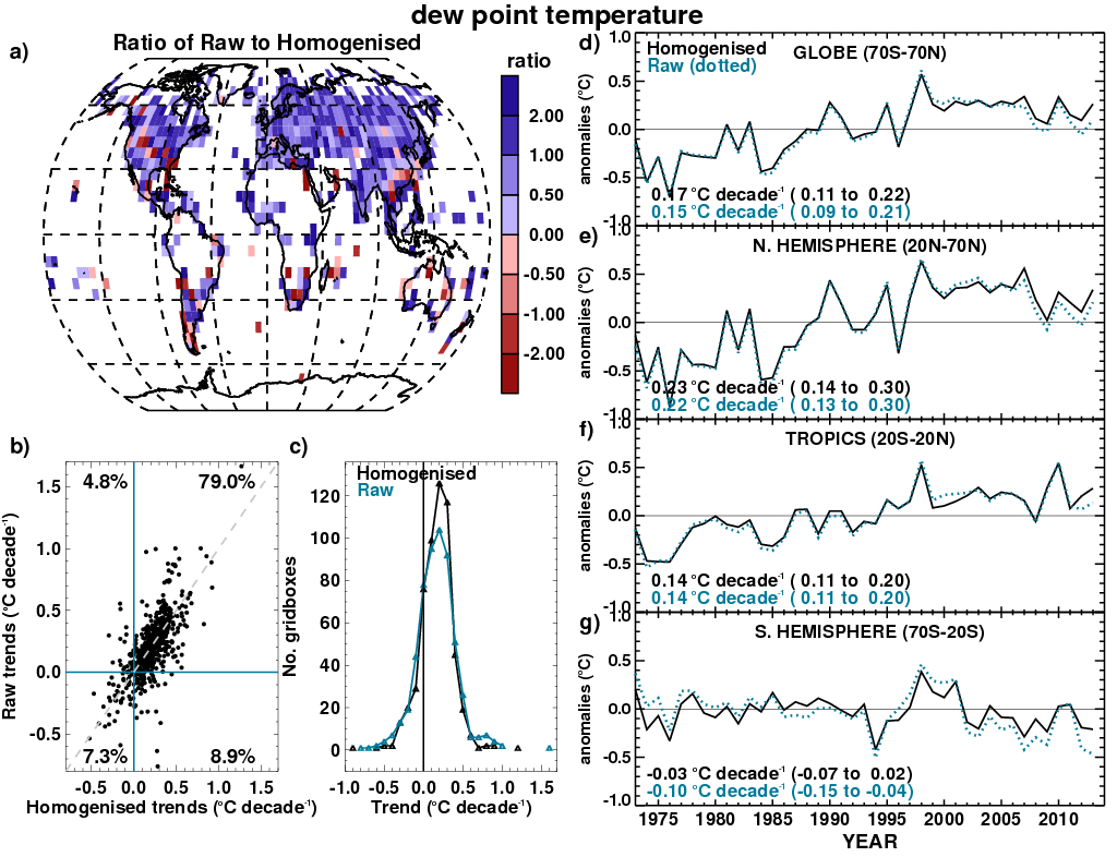
Fig. 8 Comparing raw and homogenised trends in dew point temperature	Comparison of decadal trends from 1973-2013 between raw and homogenised monthly mean dew point temperature. (a) Ratio of raw to homogenised trends for each grid box (a value of > 1 means that the raw trend is greater than the homogenised trend). (b) Scatter plot of raw verses homogenised decadal trends for each grid box with percentage presence in each quadrant. (c) Trend size distribution for raw and homogenised grid boxes. (d) Large-scale area-average time series (weighted by the cosine of the latitude) and decadal trends calculated using the median of pairwise slopes with 5th to 95th percentile slopes as con?dence intervals.	Fig8_HadISDH.landTd.2.0.0.2013p_FLATgridPHADPD5by5_MAY2014_MPtrendsscat_19732013_v1.png
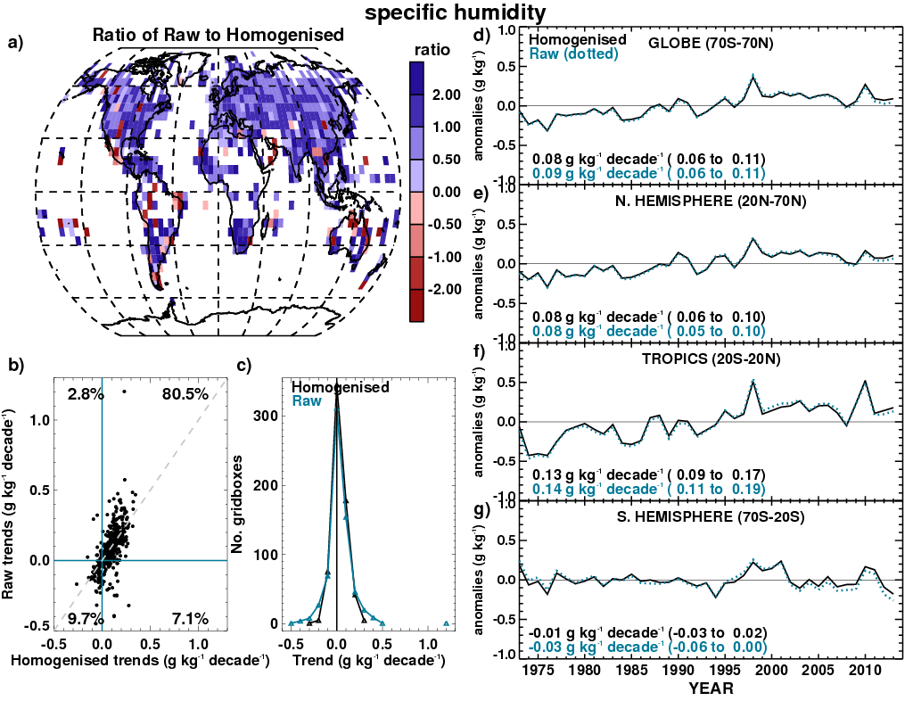
Fig. 9 Comparing raw and homogenised trends in specific humidity	Comparison of decadal trends from 1973-2013 between raw and homogenised monthly mean specific humidity. (a) Ratio of raw to homogenised trends for each grid box (a value of > 1 means that the raw trend is greater than the homogenised trend). (b) Scatter plot of raw verses homogenised decadal trends for each grid box with percentage presence in each quadrant. (c) Trend size distribution for raw and homogenised grid boxes. (d) Large-scale area-average time series (weighted by the cosine of the latitude) and decadal trends calculated using the median of pairwise slopes with 5th to 95th percentile slopes as con?dence intervals.	Fig9_HadISDH.landq.2.0.0.2013p_FLATgridIDPHA5by5_MAY2014_MPtrendsscat_19732013_v1.png
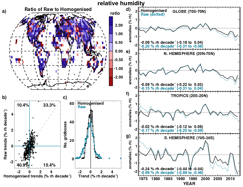
Fig. 10 Comparing raw and homogenised trends in relative humidity	Comparison of decadal trends from 1973-2013 between raw and homogenised monthly mean relative humidity. (a) Ratio of raw to homogenised trends for each grid box (a value of > 1 means that the raw trend is greater than the homogenised trend). (b) Scatter plot of raw verses homogenised decadal trends for each grid box with percentage presence in each quadrant. (c) Trend size distribution for raw and homogenised grid boxes. (d) Large-scale area-average time series (weighted by the cosine of the latitude) and decadal trends calculated using the median of pairwise slopes with 5th to 95th percentile slopes as con?dence intervals.	Fig10_HadISDH.landRH.2.0.0.2013p_FLATgridIDPHA5by5_MAY2014_MPtrendsscat_19732013_v1.png
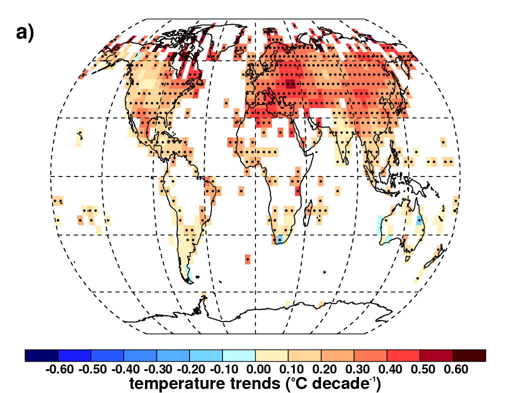
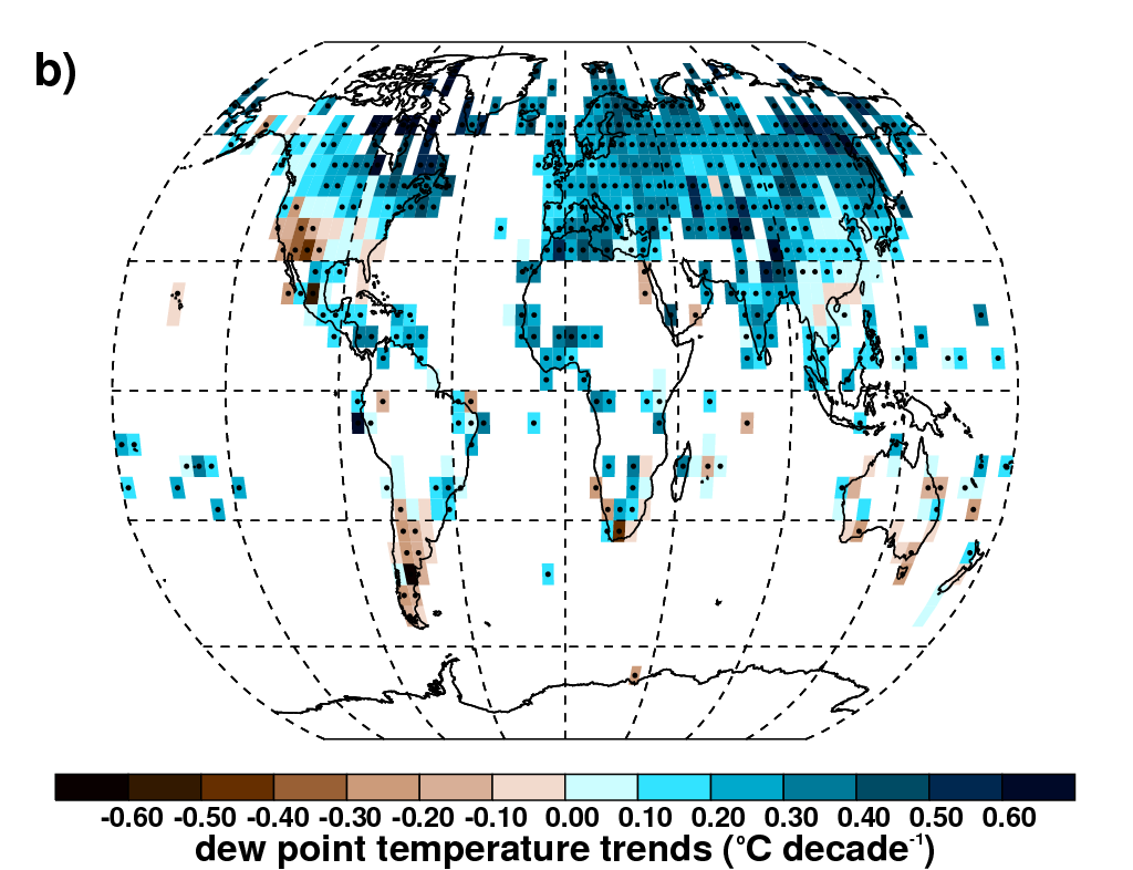
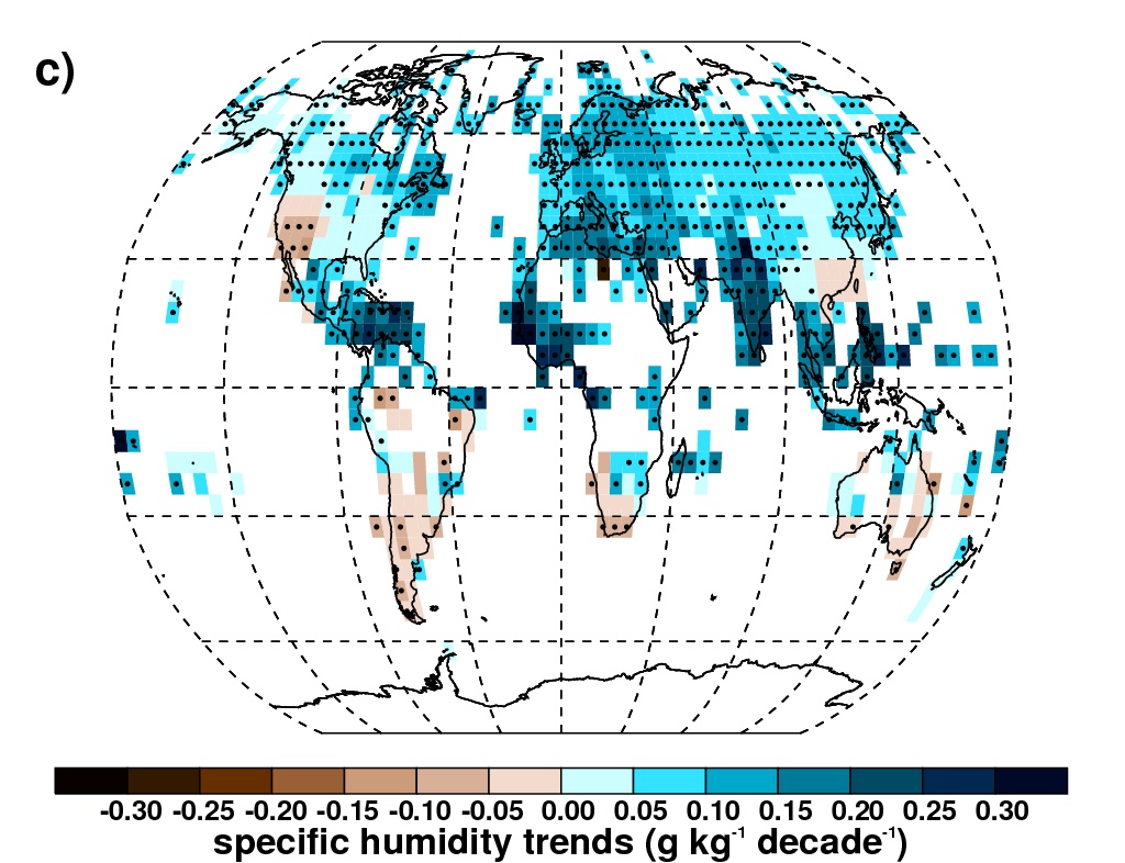
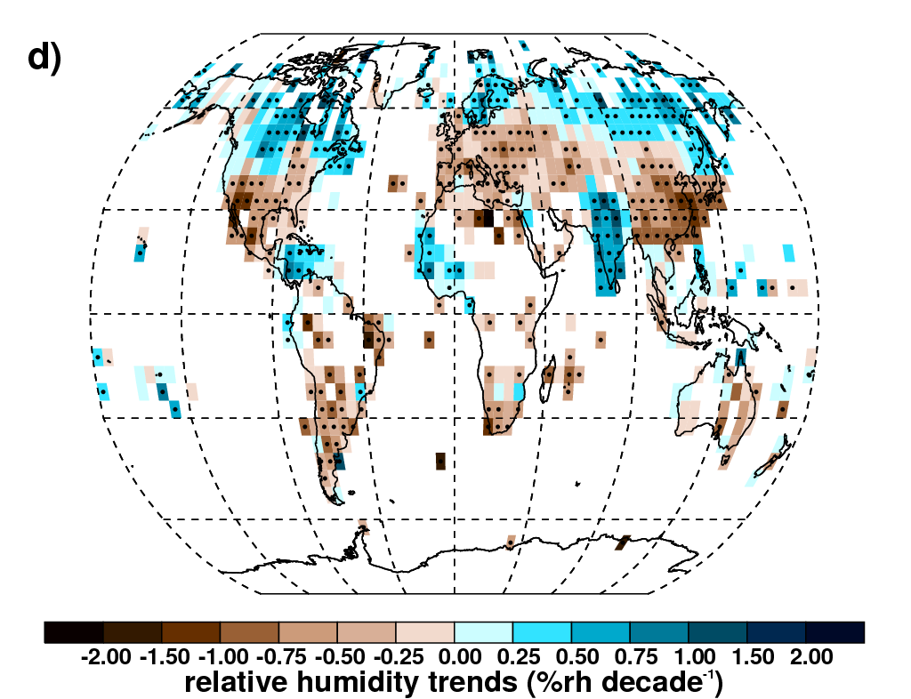
Fig. 11 Gridbox decadal trends 1973-2013	Decadal trends from 1973-2013 for monthly mean climate anomalies relative to 1976-2005. Trends are ?tted using the median of pairwise slopes. Black dots show trends that are considered to be significantly different from a zero trend where the 5th and 95th percentiles of the pairwise slopes are in the same direction. (a) Temperature, (b) dew point temperature, (c) specific humidity and (d) relative humidity. See Fig. SM6 for other variables.	Fig11a_HadISDH.landT.2.0.0.2013p_FLATgridIDPHA5by5_SEP2014_MPdectrends_19732013_v1.png, Fig11b_HadISDH.landTd.2.0.0.2013p_FLATgridPHADPD5by5_SEP2014_MPdectrends_19732013_v1.png, Fig11c_HadISDH.landq.2.0.0.2013p_FLATgridIDPHA5by5_SEP2014_MPdectrends_19732013_v1.png, Fig11d_HadISDH.landRH.2.0.0.2013p_FLATgridIDPHA5by5_SEP2014_MPdectrends_19732013_v1.png,
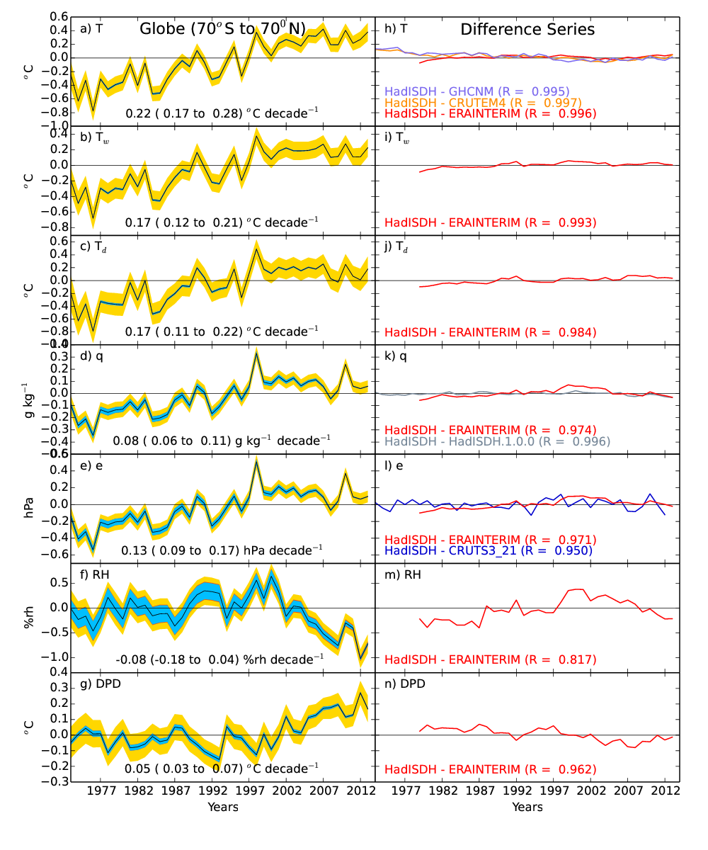
Fig. 12 Global average time series	Comparison global (70° N to 70° S) average time series of annual mean climate anomalies from HadISDH.2.0.0 with difference series for other monitoring products spatially matched to HadISDH grid box size and coverage. HadISDH uncertainty ranges for station (blue), sampling (red) and coverage (gold) uncertainty contributions combined are shown. All series have been given a zero mean over the common 1981-2010 period. Decadal trends with 5th to 95th percentile confidence ranges are shown for HadISDH and correlation coeficients of the standardised climate anomalies (not detrended) are shown. (a, h) Temperature, (b, i) wet bulb temperature, (c, j) dew point temperature, (d, k) specific humidity, (e, l) vapour pressure, (f, m) relative humidity, (g, n) dew point depression.	Fig12_PlotCompsTimeSeries.2.0.0.2013p_annual_SEP2014_v1.png
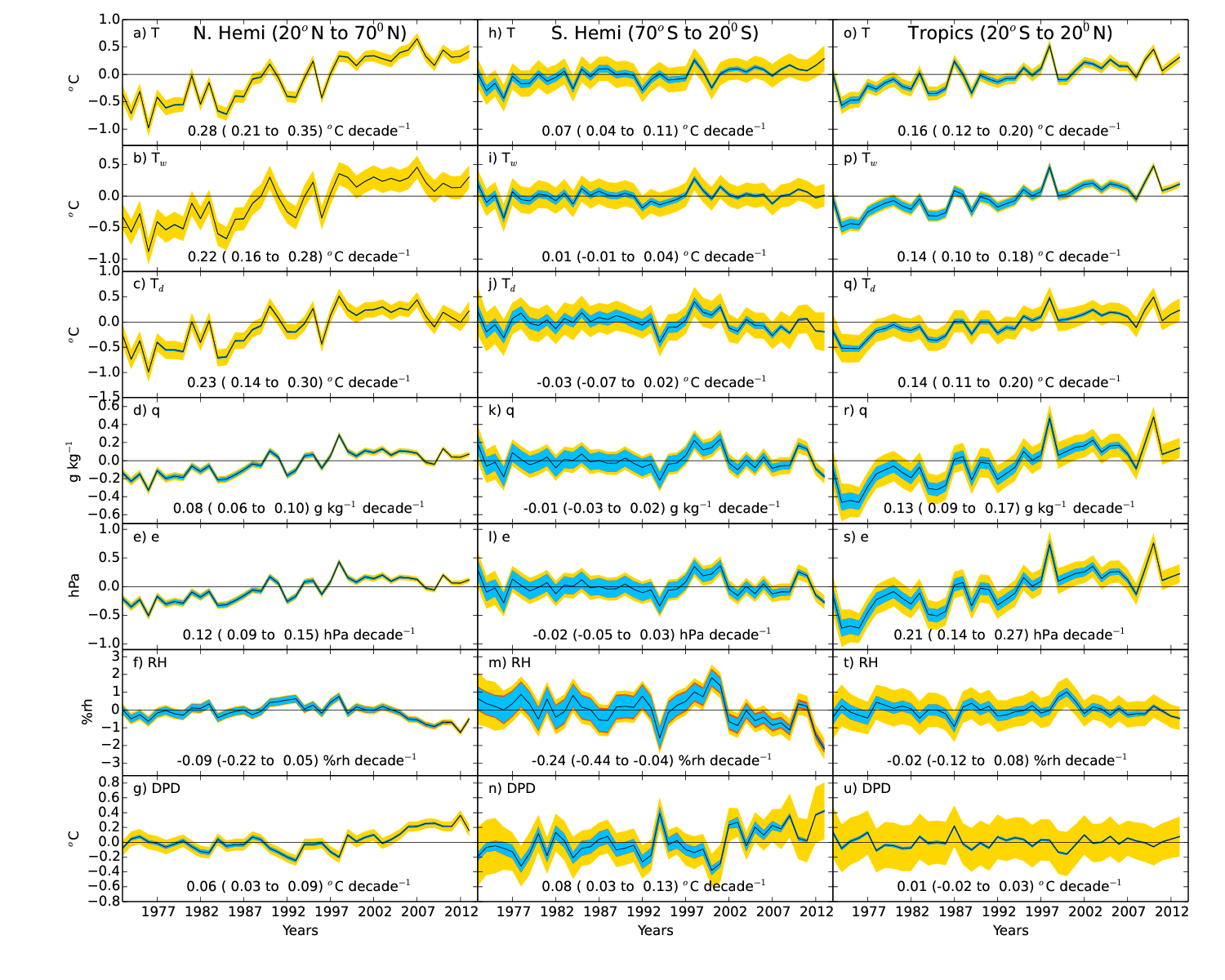
Fig. 13 Regional average time series	HadISDH.2.0.0 regional average time series for all variables for with combined uncertainties broken down by coverage (gold), temporal sampling (red) and station (gold). Decadal trends are shown with 5th to 95th percentile confidence intervals. (a, h, o) Temperature, (b, i, p) wet bulb temperature, (c, j, q) dew point temperature, (d, k, r) specific humidity, (e, l, s) vapour pressure, (f, m ,t) relative humidity, (g, n, u) dew point depression.	Fig13_PlotRegionsTimeSeries.2.0.0.2013p_annual_MAY2014_v1.png

Further plots and text will appear here over time