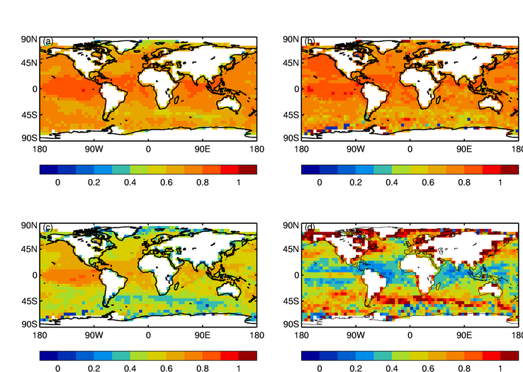
Part 1, Figure 1: (a) r_space, (b) r_time, (c) r_all and (d) sqrt(sigma_s^2(1-r))) the sampling error (°C) on a single observation.
| Met Office Hadley Centre observations datasets |
| > Home > Next page > |
Part 1, Figure 1: (a) r_space, (b) r_time, (c) r_all and (d) sqrt(sigma_s^2(1-r))) the sampling error (°C) on a single observation.
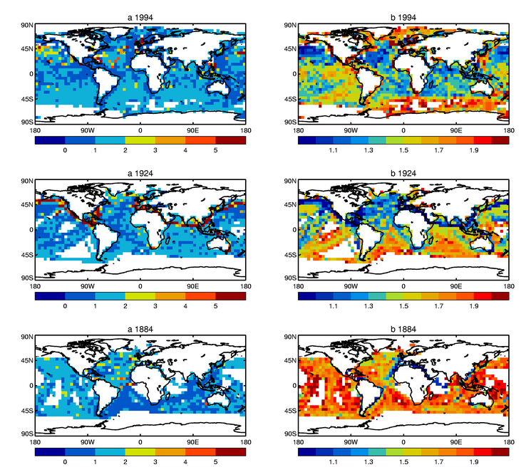
Part 1, Figure 2: Values of a (left) and b (right) calculated for three different nine-year periods centred on: 1994(top), 1924 (middle) and 1894 (bottom). a and b are dimensionless quantities.
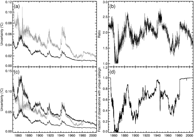
Part 1, Figure 3: (a) Uncertainty of global monthly average SST anomaly for the error model including inter-grid box correlations (grey) and for the error model with no inter-grid box correlations (black). (b) Ratio of the two lines in panel (a). (c) as for panel (a) but including an estimate of the full uncertainty of the global monthly average SST anomaly (upper black line). This is 2.4 times the lower black line prior to 1982 and equal to the grey line after 1982. (d) Fraction of observations with unique call signs.
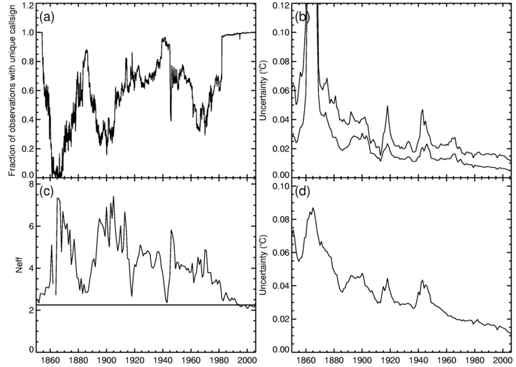
Part 1, Figure 4: (a) fraction of observations in each month from 1850 to 2006 with unique call signs. (b) Uncertainty of the global annual average sea-surface temperature calculated from only those observations with unique call signs. The upper line shows the full error calculation described in Section 4.3, and the lower line was calculated from the uncertainties on the monthly averages assuming that they are independent. (c) N_eff calculated from the uncertainties shown in panel (b). The horizontal line is at N_eff=2.25. (d) The uncertainty of the global annual average sea-surface temperature calculated using all observations and assuming N_eff=2.25.
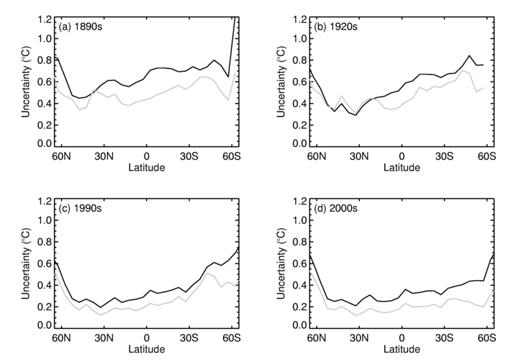
Part 1, Figure 5: Zonal average of 5° latitude by 5° longitude grid box 1-sigma uncertainties (°C) for: (a) 1890s, (b) 1920s, (c) 1990s and (d) 2000-2006. The black line is the new estimate of the uncertainty and the grey line is the estimate from Rayner et al. (2006).
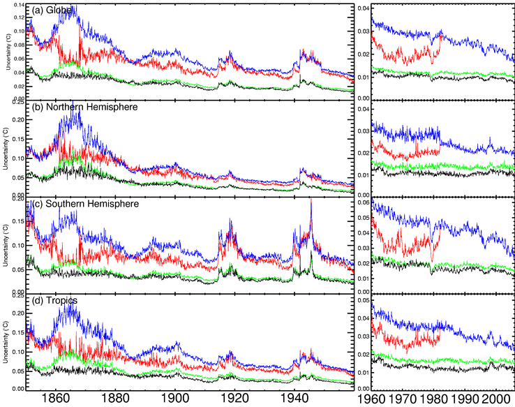
Part 1, Figure 6: 1-sigma uncertainties on monthly SSTs for (a) Global-, (b) Northern Hemisphere-, (c) Southern Hemisphere- and (d) Tropical-averages. The blue line shows the uncertainty calculated using the full error model including inter grid box correlations corrected for missing callsigns. The red line shows the uncertainty calculated using the full error model including inter grid box correlations, but not corrected for missing call signs. The green line shows the uncertainty if the grid-box errors are assumed to be uncorrelated. The lower black line is the Rayner et al. (2006) estimate. Note the different scales on each diagram. The right hand column is shown on an expanded scale because the uncertainties are generally smaller in the later period.
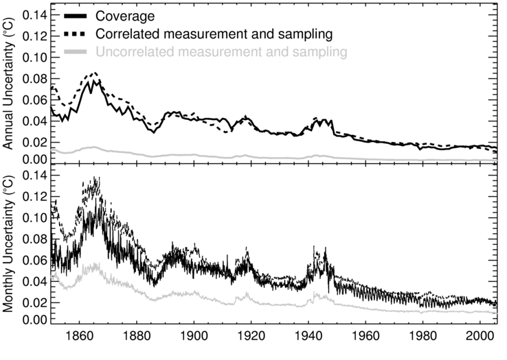
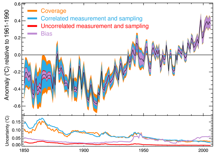
Part 1, Figure 7: 1-sigma uncertainties of annual-average (upper panel) and monthly-average (lower panel) global SST anomalies. The three lines in each panel correspond to the coverage uncertainty (solid black line), the correlated measurement and sampling uncertainty (dashed black line) and the uncorrelated measurement and sampling uncertainty (solid grey line).
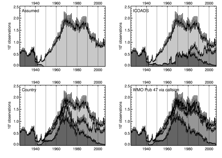
Part 2, Figure 1: Numbers of SST observations from ships for different measurement methods (1925-2006). Buckets (dark grey), ERI and Hull Contact sensors (mid grey), unknown (light grey). (top left) Observations identified by default: i.e. all observations prior to 1941 are bucket observations unless otherwise stated, Royal Navy observations from World War 2 are ERI measurements. (top right) observations identified using information in ICOADS and by default. (bottom left) observations identified using country information, ICOADS and by default. (bottom right) observations identified using all methods.
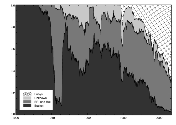
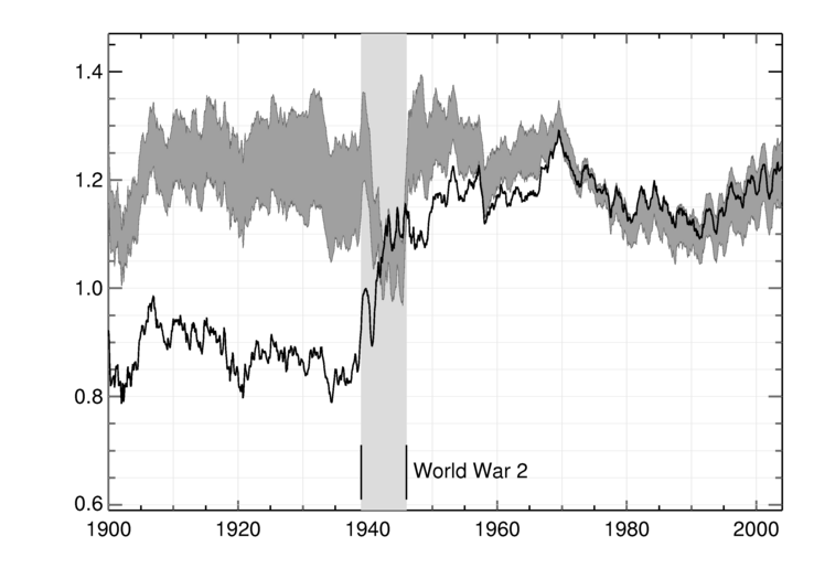
Part 2, Figure 2: Fractional contribution to the monthly global-average SST from different measurement methods and platforms (1920-2006): buckets (dark grey), ERI and hull contact (mid grey), Unknown (pale grey) and buoys (cross-hatched). The global-average SST anomaly is effectively a weighted sum of all available observations. The fractional contribution for a given measurement method was calculated as the sum of weights for that observation type.
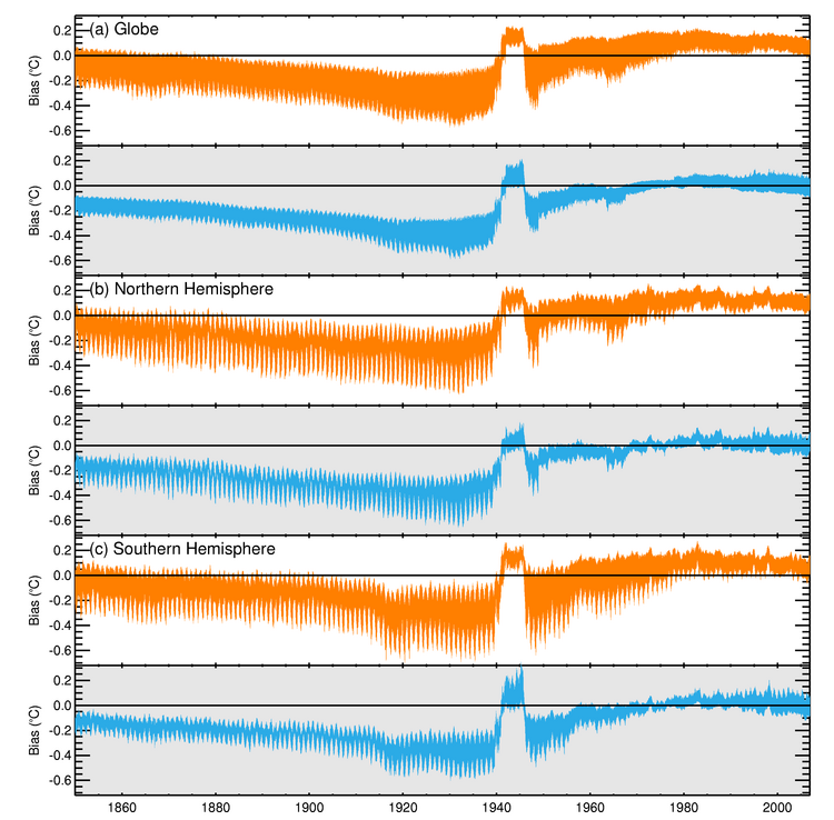
Part 2, Figure 3: 100 realisations of the monthly biases in the (a) global average, (b) northern-hemisphere average and (c) southern-hemisphere average. The shaded areas represent the 99\% uncertainty range of the estimates. The orange areas show the estimated bias relative to the true SST and the blue areas show the bias relative to the average bias for the period 1961-1990 (b-b_bar from Equation 10)
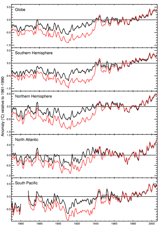
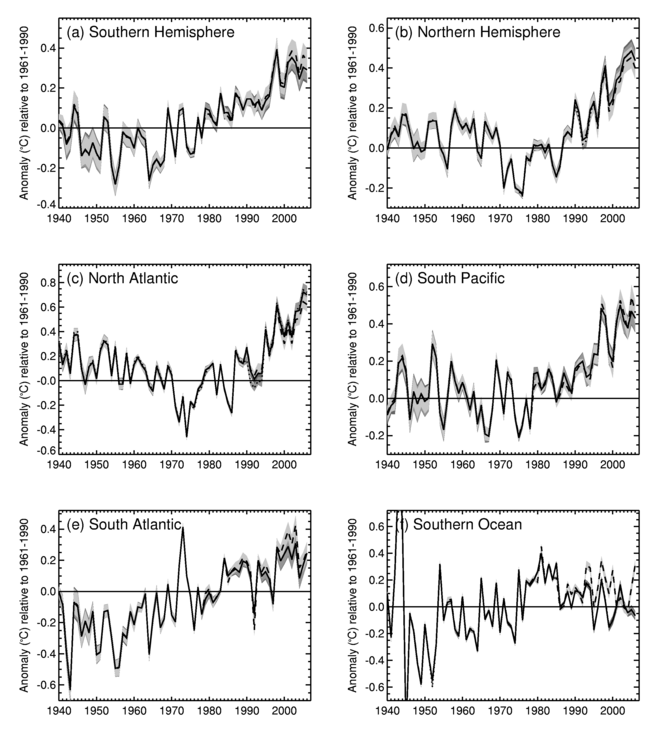
Part 2, Figure 4: Regional annual-average SST anomalies 1850-2006 (relative to 1961-1990) for 100 realisations of HadSST3 (black line plus 2 standard deviations grey area) and unadjusted gridded data (red line).
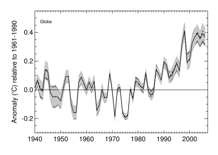
Part 2, Figure 5: Global-average SST anomalies 1940-2006 for 100 realisations of each of the different bias adjustment methods. The solid line is the original method (MAIN_SET). The dashed line is from the method based only on ship data (SHIP_ONLY). The dotted line uses the alternative method based on drifting buoy data (BUOY_FIXED). The grey areas show the 2-sigma uncertainty ranges for the three data sets.
Part 2, Figure 6: Area-average SST anomalies 1940-2006 for 100 realisations of the three different bias adjustment methods. The solid line is the original method (MAIN_SET). The dashed line is from the method based only on ship data (SHIP_ONLY). The dotted line uses the alternative method based on drifting buoy data (BUOY_FIXED). The grey areas show the 2-sigma uncertainty ranges for the three data sets.
Part 2, Figure 7: Global annual average sea surface temperature anomalies 1945-2006 from ERI measurements (orange), bucket measurements (blue), buoy measurements (red) and from all observations (black). Unadjusted series are shown in the upper panel and 100 realisations of the adjusted series are shown in the lower panel. The black line in the upper panel is duplicated in the lower panel for comparison. The ERI and bucket observations have been colocated and the buoy observations have been reduced to the common coverage of the bucket and ERI observations. At some times the buoy data have a lower coverage than the colocated ERI and bucket observations. The black lines showing averages based on all observations are also colocated with the ERI-only and bucket-only data.
Part 2, Figure 8: Southern hemisphere annual average sea-surface temperature anomalies 1945-2006 from ERI measurements (orange), bucket measurements (blue), buoy measurements (red) and from all observations (black). Unadjusted series are shown in the upper panel and 100 realisations of the adjusted series are shown in the lower panel. The black line in the upper panel is duplicated in the lower panel for comparison. The ERI and bucket observations have been colocated and the buoy observations have been reduced to the common coverage of the bucket and ERI observations. At some times the buoy data have a lower coverage than the colocated ERI and bucket observations. The black lines showing averages based on all observations are also colocated with the ERI-only and bucket-only data.
Part 2, Figure 9: Northern hemisphere annual average sea surface temperature anomalies 1945-2006 from ERI measurements (orange), bucket measurements (blue), buoy measurements (red) and from all observations (black). Unadjusted series are shown in the upper panel and 100 realisations of the adjusted series are shown in the lower panel. The black line in the upper panel is duplicated in the lower panel for comparison. The ERI and bucket observations have been colocated and the buoy observations have been reduced to the common coverage of the bucket and ERI observations. At some times the buoy data have a lower coverage than the colocated ERI and bucket observations. The black lines showing averages based on all observations are also colocated with the ERI-only and bucket-only data.
Part 2, Figure 10: The time series show the annual average area-weighted regression coefficient of the monthly average air sea temperature difference on the climatological average difference. Values are scaled by the 60°S-60°N average air-sea temperature difference to give values with units of degrees Celsius (cf Smith and Reynolds (2002), Fig. 4b). 100 realisations of the bias adjusted data are shown as the dark grey area and the unadjusted data are shown in black. The pale grey area shows the period during the Second World War when the NMAT observations are adjusted using DMAT observations.
Part 2, Figure 11: Global-average SST anomaly (relative to 1961-1990) showing the cumulative effect of adding different error components (coloured areas): median HadSST3 value (black) 2-sigma uncertainty arising from assumptions in bias adjustments (purple); measurement and sampling error, assuming these are uncorrelated between grid boxes (red); and the uncertainty including the inter-grid box correlations (blue) and the total uncertainty including all the above terms and the coverage uncertainty (orange). The lower panel shows the sizes of the individual components as 2-sigma uncertainties.
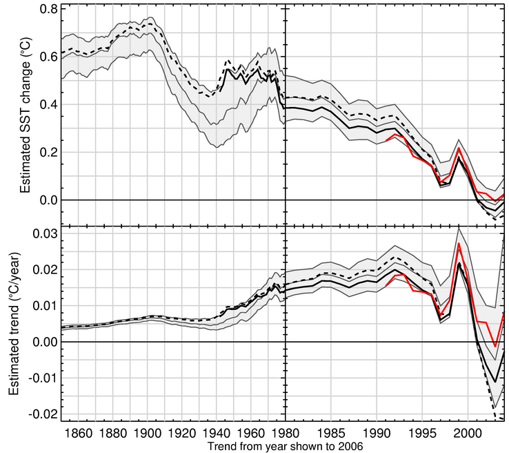
Part 2, Figure 12: (upper panel) Estimated changes in annual global-average SST calculated by multiplying the Ordinary Least Squares trend (estimated over the period starting at the year shown on the x-axis and ending in 2006) by the length of the period. (lower panel) Estimated OLS trend. The left hand panels shows start dates between 1850 and 1980 and the right hand panels shows start dates between 1980 and 2006 on an expanded scale. The solid black line shows the gridded unadjusted ICOADS 2.5 data (from 1942). The dashed black line shows HadSST2. The grey area and lines show the median and range of the 100 realisations of HadSST3. The red line shows unadjusted data from buoys only. Note that the data are not colocated so there are large differences in coverage between buoy data and all data prior to around 1997.
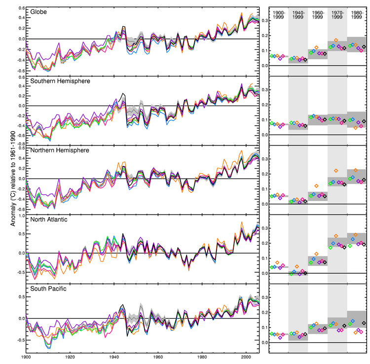
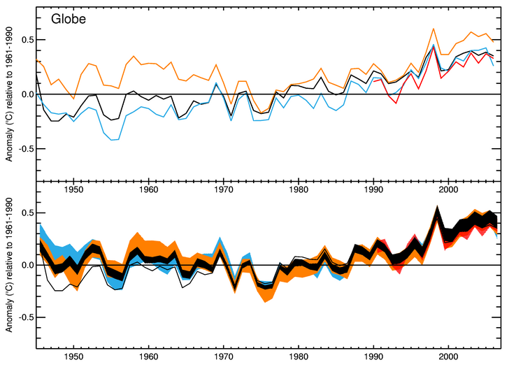
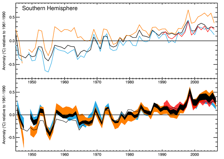
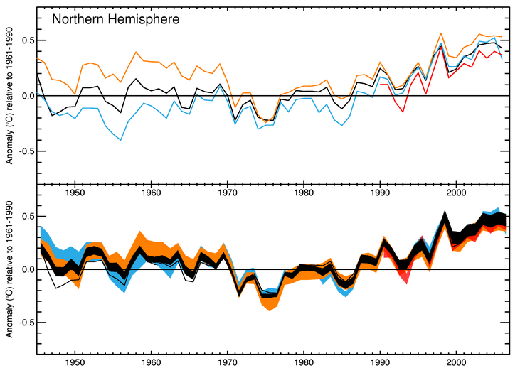
Part 2, Figure 13: Global- and regional-average marine temperature anomalies 1900-2006 (relative to 1961-1990) from the ERSSTv3 analysis (green), HadSST2 (blue), MOHMAT (orange), Kaplan SST (purple), COBE (pink), ICOADS summaries (1941-2006 only, black) and HadSST3 (grey area). All data sets have been reduced to have the same coverage as HadSST3. The panels on the right show trends (°C/decade) for the periods: 1900-1999, 1940-1999, 1960-1999, 1970-1999 and 1980-1999 from the same data sets.
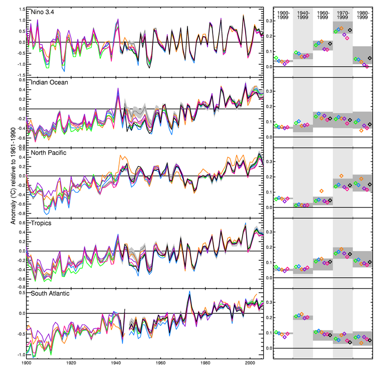
Part 2, Figure 14: Regional-average marine temperature anomalies 1900-2006 (relative to 1961-1990) from the ERSSTv3 analysis (green), HadSST2 (blue), MOHMAT (orange), Kaplan SST (purple), COBE (pink), ICOADS summaries (1941-2006 only, black) and HadSST3 (grey area). All data sets have been reduced to have the same coverage as HadSST3. The panels on the right show trends (°C/decade) for the periods: 1900-1999, 1940-1999, 1960-1999, 1970-1999 and 1980-1999 from the same data sets.
Commercial and media enquiriesYou can access the Met Office Customer Centre, any time of the day or night by phone, fax or e-mail. Trained staff will help you find the information or products that are right for you. |
 |
Maintained by: John Kennedy |
© Crown Copyright
|