
New radar noise level estimator
March 2019 - The Met Office have successfully implemented a new scheme to measure the noise power of the weather radar receiver.
Introduction
The Met Office maintains and regularly upgrades the UK Weather Radar Network, with continuous in-house research and development efforts. As part of an on-going collaboration with the National Severe Storms Laboratory in the US, we have successfully implemented their scheme to measure the noise power of the weather radar receiver. This is used in estimating the true strength from rainfall echoes (noise subtraction), as well as in estimating the amount of signal attenuation by heavy rainfall. This improvement should lead to better data quality overall and thus a more accurate rainfall rate estimate.
What is a weather radar receiver?
A weather radar receiver is essentially a device for measuring the power reflected from a region of liquid or frozen water at radio frequency. Like any radio receiver, it measures not only the reflected power, but also any additional noise from the atmosphere, the ground, the sun and artificial radio emitters, as well as introducing some electronic noise due to thermal effects in its own circuits.
This noise power results in an increase in the power measured by the radar, and it is always present in every measurement volume, whether or not there is a physical target returning a radar echo. This noise power must be subtracted from the receiver measurements to yield the actual strength of the echo. In the past, the Met Office weather radar software has relied on making hundreds of measurements at long range (beyond 300 km) from the radar, and averaging these to estimate the noise power. At this long range, it is assumed that the radar beam has cleared the troposphere, and there are no further targets, meteorological or otherwise, contributing to the measurements. The noise power should therefore be the only thing contributing to the measurements beyond this distance.
In practise, under conditions known as anomalous propagation, the radar beam can be refracted closer to the ground than usual, and thus the long range measurements can start to sample distant weather events or the beam can even be refracted back towards the ground again. Even during normal propagation, there is often contamination from aircrafts or artificial radio sources.
A key benefit of developing and running the entire UK Weather Radar network in-house at the Met Office is that we are able to develop and implement new ideas easily, and test them on an operational-standard experimental radar (Wardon Hill), thus improving the speed with which research and development can be taken from the lab and into operations.
For some time now, the Met Office radar team has been working in close collaboration with the Cooperative Institute for Mesoscale Meteorological Studies (CIMMS), which is a collaboration between the University of Oklahoma, and NOAA's National Severe Storms Laboratory (NSSL). The new range-independent radial noise estimator was developed by Igor Ivić et al. in 2012, and was transfered to the Met Office as part of this collaboration in 2017. It has been running on the UK Weather Radar Network since mid-December 2018.
The new scheme
In the following figure, the gray line (top and bottom panels on the left) represents the data along a single radial (i.e. 1° in azimuth). The horizontal axis represents distance and the vertical axis represents the power measurements from the radar receiver along this radial (in analog to digital converter "counts", which is proportional to the power before calibration). The black dots represent the data used by the long range noise estimator (top panel), and the dashed line represents the result of that estimate. There is a point contamination at about 390 km from the radar, which biases the estimate very slightly. The histogram (top right panel) is nearly Gaussian in its general shape, and the mean appears reasonable, but the spread is much larger than expected, because the standard deviation is sensitive to the outliers.
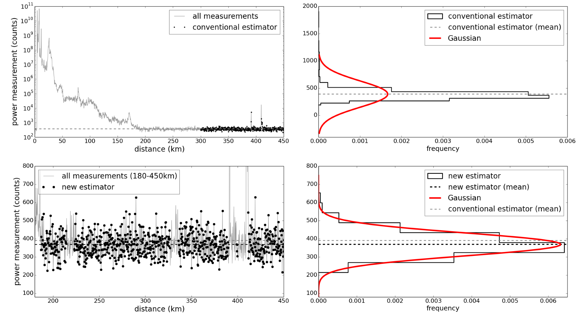 Top left: Power measurements along a single radial, with the data used by the conventional estimator shown in black. Top right: A histogram of the data used by the conventional estimator (black), the noise power estimate (dashed gray line) and a theoretical Gaussian distribution for the estimate (red). Bottom left: All the measurements between 180 and 450 km, with the data selected by the new estimator shown in black. Bottom right: A histogram of the data selected by the new scheme (solid black), with the dashed line (black) representing the mean from the new scheme (the old estimate is shown by the dashed gray line for comparison). The red curve is a theoretical Gaussian distribution for the new estimate.
The new scheme works in a similar way that a human expert would approach the problem: they would attempt to fit a horizontal line that closely represents the continuous regions of lowest power. The new scheme achieves this by characterising the statistical structure of the background noise. Generally, a series of measurements of pure noise would be distributed according to a Gaussian distribution. Signals from other sources (contamination in this case) would tend to be highly correlated and would thus be expected to deviate from this Gaussian distribution. The new scheme uses a series of steps where it detects segments of the data with signals in them, censors these segments, and iteratively continues to look for signals in the remaining data. The steps are described in detail in the original paper.
In some steps, the nearest two neighbouring measurements are used, whereas in other steps, up to 16 neighbours on each side are used. Several properties of a Gaussian distribution are considered in turn, for example, how often is a single value larger than the mean, how often does a sample of 10 pixels in a row have a variance larger than a certain threshold, how often do 10 pixels in a row lie above the median, etc. At each step, some measurements are censored because they show such high individual deviations or such high correlation that they are unlikely to have been drawn from a Gaussian distribution. As more and more measurements are censored, the remaining measurements are more closely described by a Gaussian distribution, until all that remains is noise data. At this point, any data that could have come from a non-Gaussian source have been censored.
In the bottom panels in the figure above, the new scheme is shown to pick data closer to the radar than the long range noise estimate (about 200 km instead of the fixed 300 km range), but it successfully avoids the outliers. This is reflected in the histogram in the bottom right panel, where the selected data has a histogram that is much closer to a Gaussian distribution. The conventional estimator arrived at 390 (analog to digital) counts, whereas the new estimator obtained 369 counts. The new estimate of the noise power isn't significantly different — this is an easy case, without significant contamination. This demonstrates that the new scheme is able to perform at least as well as the existing scheme in normal conditions, while showing better skill at rejecting outliers.
A more interesting case
In contrast to the above example, in the following case there is significant contamination from a pulsed source of radio interference (top left). The real noise power is somewhere in the bottom segments of the black dots, whereas the higher segments are part of the contamination. This biases the estimate significantly. Notice also that the histogram is significantly non-Gaussian (top right), due to this contamination.
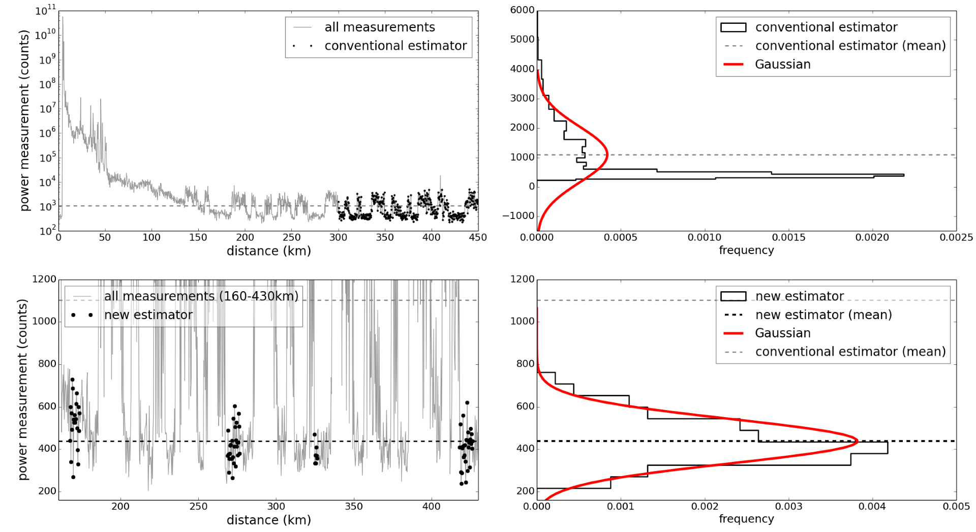 Top left: Power measurements along a single radial, with the data used by the conventional estimator shown in black. Top right: A histogram of the data used by the conventional estimator (black), the noise power estimate (dashed gray line) and a theoretical Gaussian distribution for the estimate (red). Bottom left: All the measurements between 160 and 430 km (gray), with the data selected by the new estimator shown in black. Bottom right: A histogram of the data selected by the new scheme (solid black), with the dashed line (black) representing the mean from the new scheme (the old estimate is shown by the dashed gray line for comparison — note the significant difference!). The red curve is a theoretical Gaussian distribution for the new estimate.
We can see in the bottom right panel that the new scheme has rejected all the data in the segments where the pulsed interference was strong but kept the data in the segments where the pulsed interference was absent. This is exactly what a human expert would have done, keeping the uncontaminated measurements at the expense of the contaminated ones.
In addition, the new scheme has again elected to retain some data that is closer than the usual 300km from the radar. This means we are now have more data to make the noise power estimate, because we can confidently reject any contaminating signals that might be present at closer range. Where the conventional estimator calculated 1096 counts, the new estimator came up with 446 counts, which is more realistic. In addition, the histogram shows that the data has a distribution that is much closer to a Gaussian, which reinforces our confidence that the estimate is based on the noise power contribution alone.
The overall improvement
The following figure shows the noise estimate using the conventional noise estimator or long range noise (left), using the new scheme (center), and the difference between the two (right) in digital counts (before calibration) from the receiver. The vertical axis shows scan number (i.e. over time) and the horizontal axis shows azimuth (degrees).
The new scheme removes the speckles from point contamination, as well as the larger and darker smudges which represent echoes from long range storms (picked up because of anomalous propagation), and yet keeps the smooth signals that correspond to a genuine increase noise power due to the radiometric emissions from attenuating (heavy) rainfall. This information is itself crucial in correcting for attenuation in heavy rainfall for a more accurate quantitative precipitation estimate (QPE).
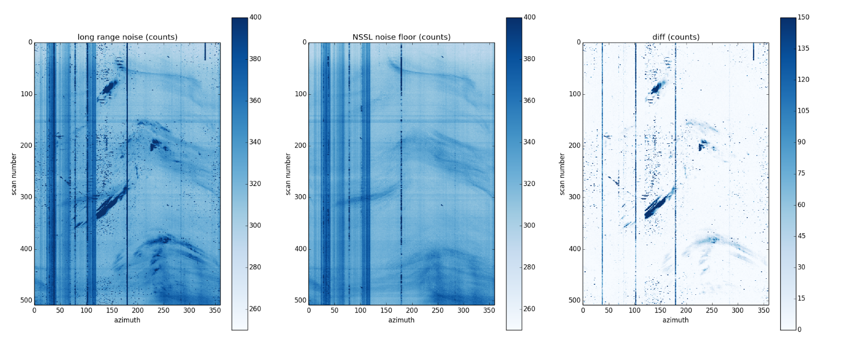 The horizontal axis is azimuth (in degrees), and the vertical axis represents time downwards, indicated with scan number (every 5 minutes). Left: Noise power estimate from the conventional estimator. Note the speckles, and various strong signals. Center:The results of the new estimator. The speckles are significantly reduced, and the dark smudges (strong contamination) are removed, whereas the smooth signals are retained - these are the radiometric emissions from radar-attenuating heavy rainfall. Right: The difference in counts (old-new) highlighting the areas where the new scheme has made an improvement.
Conclusions
As shown by the above discussion, the new scheme for measuring the weather radar noise power performs much better than the existing scheme, by approaching the problem with the same general rules that a human expert would follow. It looks for segments of data that are on average flat, i.e. devoid of signals, and distributed according to a Gaussian, and picks the segment with the lowest mean. In every case we have looked at, the new scheme estimated the same noise power that a human expert could come up with, i.e. as good as or better than the existing scheme.
The success of this project also shows both the benefits of international collaborations such as the one between the Met Office and CIMMS/NSSL, as well as the benefits of developing, maintaining and upgrading a weather radar network in-house.