Mauna Loa carbon dioxide forecast for 2026

Richard A. Betts, Chris D. Jones, Jeff R. Knight, James O. Pope and Caroline Sandford

The increase in atmospheric CO₂ at Mauna Loa is forecast to remain too fast to track IPCC scenarios that limit global warming to 1.5°C, despite being slightly slowed by a temporary strengthening of natural carbon sinks associated with moderate La Niña-like conditions in late 2025 and early 2026.

We forecast the annual average CO₂ concentration at Mauna Loa, Hawaii to be 2.37± 0.55 parts per million (ppm) higher in 2026 than in 2025. As a result, we forecast the 2026 annual average CO₂ concentration at Mauna Loa to be 429.4 ± 0.6 ppm (Figure 1). This will continue the ongoing rising trend in CO₂ seen in the long-term record of measurements from the Mauna Loa observatory in Hawaii that date back to 1958 (also known as the Keeling Curve). The Mauna Loa record is usually a good guide to rise in global average CO₂  concentration, which we therefore expect to increase by a similar amount. 

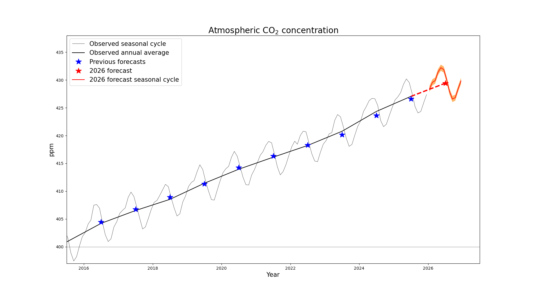
Figure 1. Forecast CO₂ concentrations at the Mauna Loa observatory, showing monthly (red curve) and annual (red star) values. The orange band and vertical red line shows the forecast uncertainty ranges. The thin and thick black curves show the observed monthly and annual average concentrations respectively. Blue stars and blue lines show previous forecast annual averages and their uncertainties, with the 2020 value being the updated 2020 forecast issued followed the reduction in global CO₂ emissions due to the Covid-19 pandemic. Observed data is from the Scripps Institution of Oceanography, UC San Diego.

The size of the annual CO₂ rise has generally been increasing but with substantial variation from year-to-year (Figure 2), with the increase from 2023 to 2024 being the largest on record. 

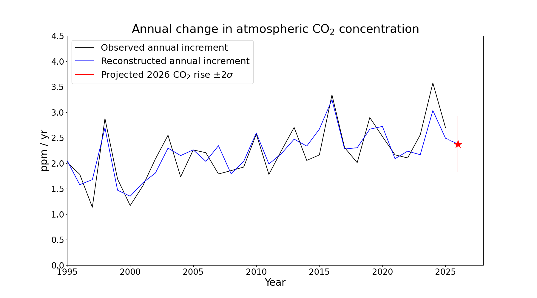
Figure 2. Annual increments in CO₂ concentration at the Mauna Loa observatory from observations (black) and the 2026 forecast (red star). The forecast uncertainty range (red line) is ± 2 standard deviations.  The blue line shows statistical reconstructions of past annual CO₂ increments using the same method as used in the forecast. Observations are from the Scripps Institution of Oceanography, UC San Diego.

Contributions of anthropogenic emissions and varying natural carbon sinks to the CO₂ rise

Long-term increases in observed CO₂ are the result of human-caused emissions of carbon dioxide into the atmosphere – more than enough CO₂ has been emitted by fossil fuel burning and deforestation to account for the increase measured in the atmosphere. Although CO₂ concentrations have now increased by over 50% since the industrial revolution, this increase would have been almost twice as large if some CO₂ had not been removed from the atmosphere through natural absorption by plants and the oceans. 

These natural sinks of carbon vary in strength from year to year due to short-term fluctuations in climate, principally linked to El Niño Southern Oscillation (ENSO) cycles in the tropical Pacific Ocean but with other aspects of climate variability also having effects. This means that although emissions are increasing relatively smoothly, the rate of CO₂ increase in the atmosphere shows more variability due to the varying strength of natural carbon sinks. El Niño conditions typically lead to a faster annual CO₂ rise, due to an overall weakening of natural carbon sinks, largely driven by hotter, drier conditions in tropical land areas. La Niña conditions have broadly opposite impacts, so typically lead to an overall strengthening of natural carbon sinks and hence a slower annual CO₂ rise. The Met Office CO₂ forecast takes account of both anthropogenic emissions and the impacts of ENSO-related climate variability on natural carbon sinks, accounting for the latter using the observed correlation between the annual CO₂ rise and sea surface temperatures (SSTs) in the equatorial Pacific Ocean (Figure 3). Producing this forecast in December, we use an annual mean SST anomaly in the Nino3.4 region combining observations from the previous April to November with a forecast from December to March. With ENSO having recently been in moderate La Niña conditions, leading to an April-March mean Nino3.4 SST anomaly of -0.46°C, we expect a temporary strengthening of carbon sinks and hence a slightly smaller rise in atmospheric CO₂ than would have been the case without this.

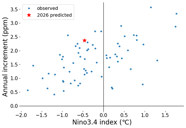
Figure 3. Annual CO₂ growth rate for years 1960 to 2025 and predicted for 2026 relative to the preceding year, vs. the Niño3.4 index for April of the preceding year to March of the current year. The Niño3.4 index is the sea surface temperature (SST) anomaly in region 5°N to 5°S and 170°W to 120°W in the Pacific Ocean, de-trended to remove the effect of long-term warming.

For short periods such as individual years, the observed rate of build-up of CO₂ in the atmosphere does not necessarily reflect changes in emissions – the effects of climate variability on the short-term rise can dominate. However, in the longer term, the ongoing increase in the annual rate of CO₂ rise is quite evident despite large interannual variability (Figure 4). When the effects of ENSO are removed, the calculated CO₂ rise shows an ongoing increase, but with the rate of increase slowing around 2012 due to the slowing of the rise in global emissions. There was also a temporary slowing of the ENSO-adjusted CO₂ rise in 2020 due to the reduction in global emissions following worldwide reductions in transport and energy production during the COVID-19 pandemic.

Impact of El Niño on the forecast CO₂ rise in 2026

We can estimate the potential contribution of the recent moderate La Niña conditions to the CO₂ rise forecast for 2026 by repeating our forecast calculation without the sea surface temperature change, ie: with "neutral" conditions. This suggests that without a La Niña response in the atmosphere and tropical land ecosystems, the forecast annual mean CO₂ rise from 2025 to 2026 would be 2.56 ppm, a slightly faster rise than the 2.37 ppm forecast when accounting for La Niña (Figure 4).

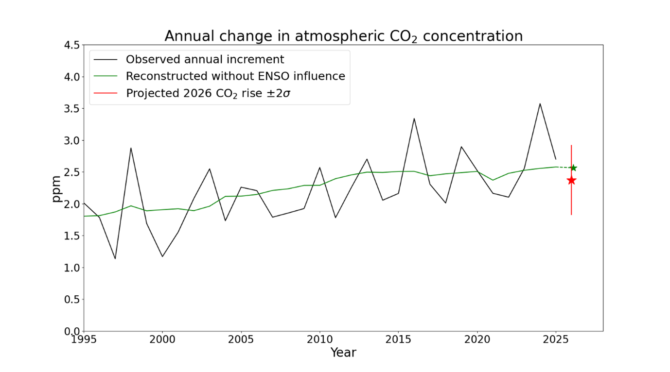
Figure 4: Annual increments in CO₂ concentration at the Mauna Loa observatory from observations (black) and the 2026 forecast (red star), and the estimated increments without the influence of ENSO (green line and green star). The forecast uncertainty range (red line) is ± 2 standard deviations.  Observations are from the Scripps Institution of Oceanography, UC San Diego.

Comparison with previous annual CO₂ increments

The average annual CO₂ rise has increased over the 6 decades of the Mauna Loa record (Table 1), due to ongoing rise in human-caused emissions, mainly due to fossil fuel burning. Despite emissions being at record high levels, the forecast rise of 2.37 ± 0.55 ppm for 2025-26 is smaller than that seen in the last 3 years due to the current La Niña conditions. The coming year’s rise is predicted be the 12th largest on record, with an uncertainty range of between the 3rd and 28th largest (Figure 5).

Table 1. Decadal average annual CO₂ rises in the Mauna Loa record

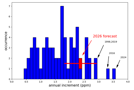
Figure 5. The central estimate of the forecast annual CO₂ increment for 2025-2026 in the context of the frequency distribution of the observed annual increment for each year in the Mauna Loa record. The horizontal red bar shows the forecast uncertainty range of ± 0.55 ppm.

Comparison with CO₂ trajectory consistent with limiting global warming to 1.5°C

The Paris Agreement commits nations to pursuing efforts to limit the rise in global temperatures to 1.5°C above pre-industrial levels. In modelled scenarios that achieve this, the rise in atmospheric CO₂ slows rapidly and ceases completely within the next two decades. The IPCC 6^th Assessment Report included 3 scenarios which have at least a 50% likelihood of limiting global warming to 1.5°C with little or no overshoot (Table 2).  The C1-IMP-LD scenario features efficient resource use and changing consumption patterns leading to low demand for resources; C1-IMP-REN focusses on renewables; and C1-IMP-SP illustrates shifting global pathways towards sustainable development. Other scenarios could also be followed, but all would require the rise in CO₂ to be slowing to zero urgently for global warming to be limited to 1.5°C, unless interventions such as solar radiation modification were assumed. 

Table 2. Decadal average CO₂ rises in three illustrative scenarios limiting global warming to 1.5° with little or no overshoot (IPCC 2022), compared with observed average in the first half of the 2020s.

The IPCC scenarios can provide a benchmark against which the observed and forecast atmospheric CO₂ rise can be compared as part of assessing progress towards the Paris Agreement goal. All three scenarios require the decadal average rate of rise in the 2020s to be slower than the rate in 2010 (1.33 to 1.79 ppm / year), but for the first 5 years of the 2020s the average rate of rise observed at Mauno Loa has been faster at 2.61 ppm / year.

Figure 6 makes a more detailed comparison with the C1-IMP-SP scenario, which is the least ambitious of the three scenarios in the near term, allowing for the fastest CO₂ rise in the 2020s. The central estimate of the forecast rise for 2025-2026 (red star) remains above the rate required to track the 1.5°C-compatible scenario, despite being smaller than the last three years. If the rise were to be at the lower end of the uncertainty range (vertical red line) then it would align with the 1.5°C scenario, but without the effects of climate variability (green star) the 2026 rise would be further above the 1.5°C scenario.  Without the small negative effect of natural climate variability, the forecast would essentially show no chance of being consistent with the 1.5°C-compatible scenario, so even the small possibility of it being consistent with this pathway is due to a temporary, reversible effect that cannot be relied upon in future years.

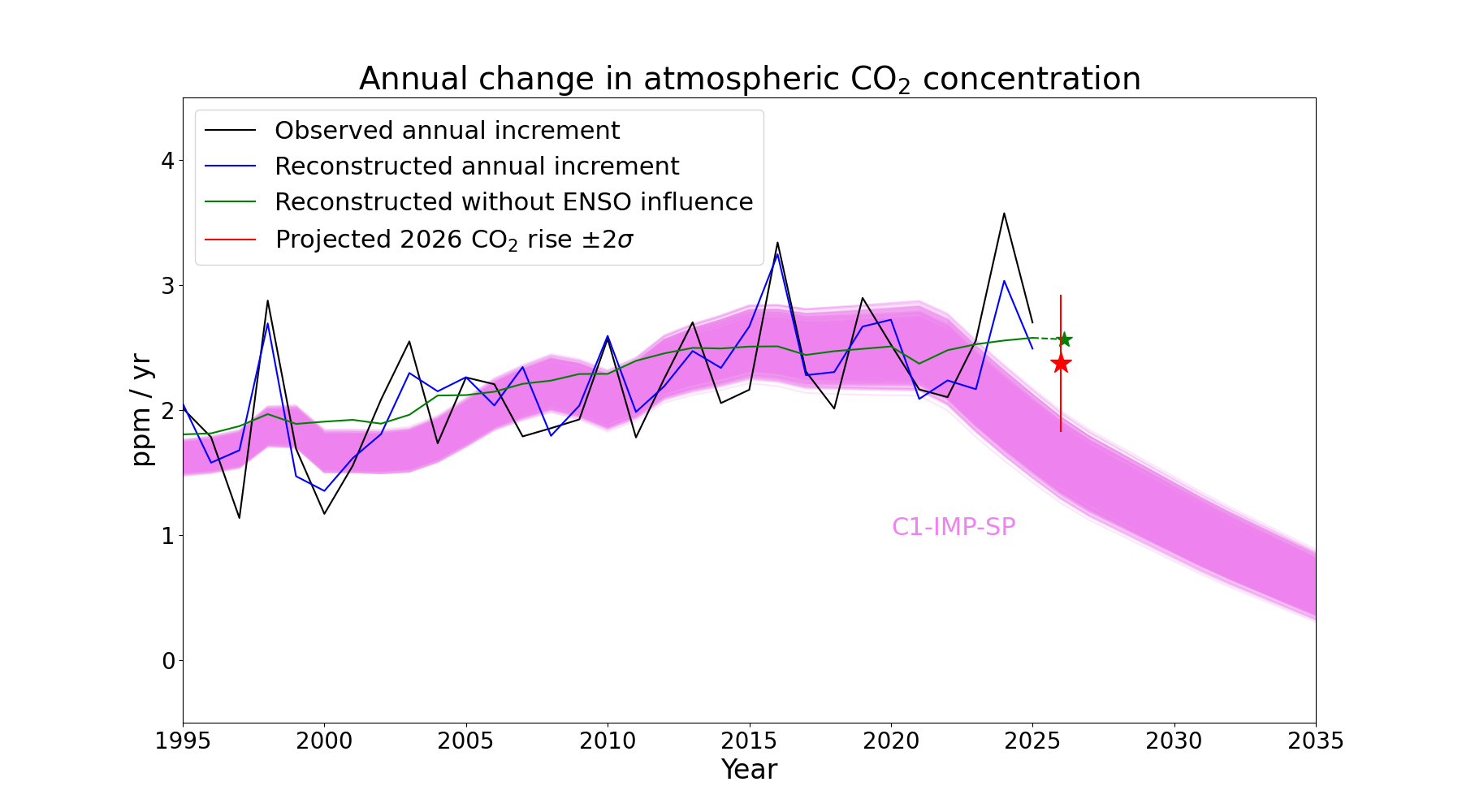
Figure 6. Comparison of recent and forecast annual CO₂ increments with an illustrative scenario limiting global warming to 1.5°C. Black line: Annual increments in CO₂ concentration at the Mauna Loa observatory from observations. Blue line: Annual increments in CO₂ concentration at the Mauna Loa observatory reconstructed using a statistical relationship between concentrations, emissions and ENSO. Red star with vertical error bars: the 2026 forecast increment. Green line and green star: Estimated increments without the influence of ENSO. Purple plume: simulated CO₂ concentrations in the C1-IMP-SP scenario limiting global warming to 1.5°C with >50% likelihood.

The extent to which the CO₂ rise would need to slow for global warming to be limited to 1.5°C can be further put into context by extending the Keeling Curve with projected concentrations from one of the illustrative 1.5°C-compatible scenarios (Figure 7). The observed rise from 2024 to 2025 is already tracking above the 1.5°C scenario, and the gap is predicted to increase in 2026.

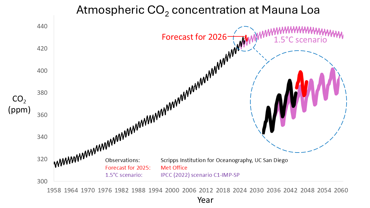
Figure 7. Monthly CO₂ concentrations from observations up to 2026 (black) and a scenario consistent with limiting global warming to 1.5°C (purple). Also shown is the Met Office forecast for 2026. Observations are the Keeling Curve record at Mauna Loa, from the Scripps Institution for Oceanography, UC San Diego, which began in March 1958. From 2024 onwards, monthly values are calculated from the annual mean concentrations in the C1-IMP-SP scenario, with an illustrative seasonal cycle imposed which continues the amplitude seen in recent years.

Seasonal cycle of CO₂ concentrations

We also predict the maximum and minimum monthly values in the seasonal cycle of CO₂ concentrations at Mauna Loa (Figure 1, Table 3).  Each year, the CO₂ value at Mauna Loa increases in the first 5 months, peaks in or around May, then declines for the next 4 months due to the uptake of CO₂ by land ecosystems in the northern hemisphere growing season.  Following a minimum, which is usually in September, atmospheric CO₂ then increases again as autumn and winter leaf-fall and decay cause a release of CO₂ back to the atmosphere. In 2026, we predict this seasonal cycle to peak at a monthly mean value of 432.2 ± 0.6 ppm in May (Figure 1, Table 3). From comparison with reconstructions of past CO₂ levels from isotopes of carbon and boron in marine sediments, this will be the highest atmospheric CO₂ concentration for over 2 million years. CO₂ will then return to a minimum monthly value of 426.6 ± 0.6 ppm in September before rising again.

Methods

The technique used to make this forecast was also used to make forecasts ahead of time for 2016, 2017, 2018, 2019, 2020, 2021, 2022, 2023, 2024 and 2025.  In 2020 we also issued an updated forecast once it became clear that the response to the Covid-19 pandemic would cause global CO₂ emissions to be much smaller than expected that year. 

Table 3. Forecast monthly average CO₂ concentrations at Mauna Loa in 2026. The 2 standard deviations uncertainty is ± 0.6 ppm

Our usual methodology uses a statistical relationship between the annual CO₂ rise, human-caused emissions and changes in sea surface temperature (SST) in the equatorial Pacific Ocean as a measure of the strength of the dominant pattern of natural climate variability that is known to affect the strength of carbon sinks. We use an average of SSTs from ocean observations in recent months and seasonal forecasts for the coming months. Previous work found that the CO₂ increment between 2 consecutive calendar years correlates most strongly with the SSTs in the 12 months from April to March within those 2 years.

For most years from 2016 to 2023, our forecast calculations used the annual emissions from the previous year as published in the Global Carbon Budget, as normally the ongoing trend in emissions is not large enough to affect the forecast substantially. Our original forecast for 2020 also made this assumption, while our revised 2020 forecast included an adjustment based on projected emissions profiles across the year applied to an atmospheric transport model. Our forecast for 2021 assumed that global emissions had returned to approximately 2019 levels, having already returned to near those levels at the end of 2020. Our forecast for 2022 used the fossil fuel emissions for 2019 and land use emissions from 2020. Our forecasts for 2023, 2024 and 2025 returned to the usual method of using Global Carbon Budget emissions from the previous year.

In our forecast we assign the same uncertainty to monthly and annual values, but this ignores the role of within-year impacts such as periods of fire activity in areas not typically affected by ENSO, or anomalous wind directions at the measurement site at Mauna Loa. Quantification of these additional sources of uncertainty at monthly levels are a topic of ongoing research and our stated uncertainty on the monthly averages will therefore be an underestimate.

Verification of the 2025 CO₂ forecast

The observed CO₂ rise of 2.68 ppm between 2024 and 2025 at Mauna Loa was larger than the central estimate of our forecast of 2.26 ppm but within the 2-sigma uncertainty of ± 0.56 ppm (Table 4). The observed monthly concentrations were higher than the central estimate of the forecast for every month except August (Figure 8, Table 5). 

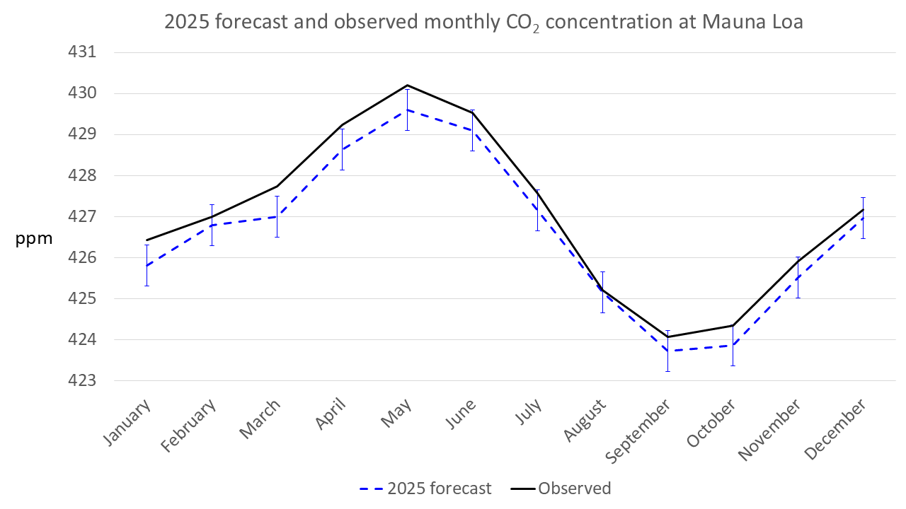
Figure 8. Comparison of Met Office forecasts of monthly CO₂ concentrations in 2025 at Mauna Loa (dashed blue line) with measurements for 2025 (solid black line) from the Scripps Institution for Oceanography UC San Diego. The vertical blue lines show the forecast uncertainty range (2 standard deviations).

Table 4. Summary of forecast and observed annual CO₂ concentrations and rises for 2016 to 2025. Note that observations were not available for December 2022 due to the eruption of the Mauna Loa volcano cutting off power supplies to the observatory, so for 2022 the comparison of forecast and observed mean concentration is given for January-November, and the forecast and observed increases are calculated relative to the January-November mean for 2021. For 2020, both the original forecast and the updated forecast accounting for the Covid-related emissions reductions are shown. 

At the time of preparing our 2025 forecast, La Niña conditions were emerging and the Niño3.4 SST anomaly was predicted to peak at around -1.0 °C in early 2025, leading to a predicted April 2024 – March 2025 anomaly of  -0.35 °C [2-sigma uncertainty -0.73 to +0.04 °C] which agreed well with the observed anomaly of -0.21 °C. Our method had therefore forecast CO₂ rise to probably be smaller than would have been expected from considering emissions alone (2.40 ppm). In contrast, the observed rise was larger than would be expected considering emissions alone (Figure 9). This may point to other processes also potentially being important for variability in the annual atmospheric CO₂ rise in addition to ENSO.

Table 5. Forecast and observed monthly average CO₂ concentrations at Mauna Loa over 2026. The uncertainty in the forecast values was ±0.6 ppm. Observed monthly averages for January to November are those published by the Scripps Institution for Oceanography at UC San Diego, and those for December are provisionally estimated from daily values reported on the Scripps social media channel.

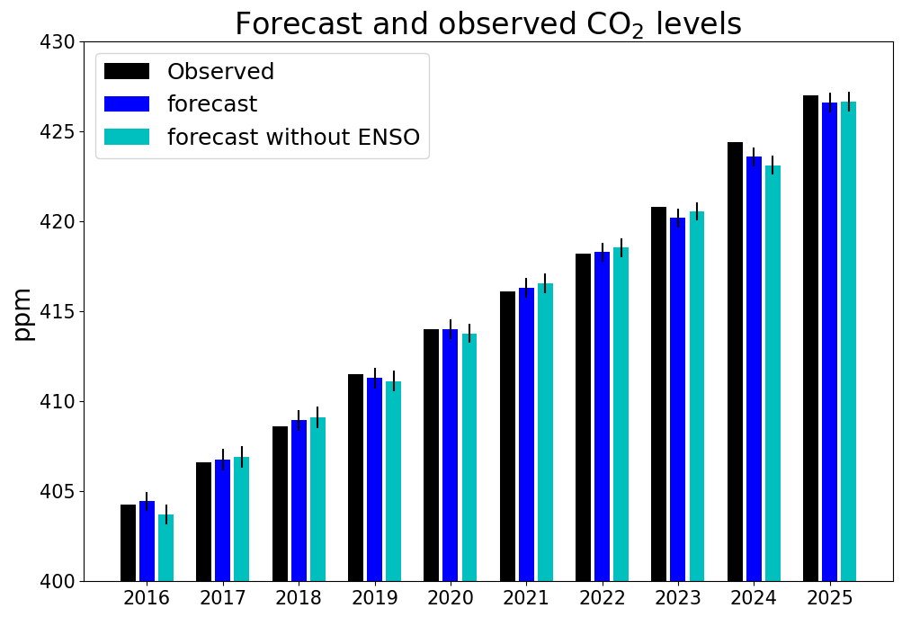
Figure 9.  Annual average CO₂ concentrations for 2016 to 2025 from observations (black) and forecasts including the statistical relationship with ENSO (dark blue) and re-forecast values based on emissions alone, without the effects of ENSO (light blue). Thin black lines show the forecast uncertainty range (2 standard deviations).

Note: definitions of annual CO₂ rise, increment and growth rate 

We define the annual CO₂ rise or annual increment for a particular year as the difference in annual average concentration for that calendar year and that of the previous calendar year.  This is different to the definition of annual 'growth rate' as published by NOAA  which is the average change across an individual calendar year.  

Acknowledgements

This work is supported by the Met Office Hadley Centre Climate Programme funded by DSIT.

Published 4th February 2026